LuciadRIA Samples
Browse samples per component: All installed
Highlighted samples
Panorama
BIM Viewer sample
Video panorama
Symbology Encoding
Data Formats
MGRS Grid
Military Symbology
Multispectral Analysis
OGC 3D Tiles
LuciadRIA
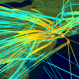
Parameterized Lines
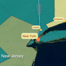
The Parameterized Lines sample illustrates how to flexibly style and filter polylines via a dedicated painter. Any attribute can be used to thematically style the data. All calculations are performed client-side.
The sample shows a dataset of flight to and from New York.
Each flight has a couple of properties:
- Id : its callsign
- Class : the class of aircraft, for example Turboprop
- Type : the aircraft type, for example Airbus A320
- Heading : the direction (azimuth)
- Speed : the speed over ground
- Climb rate : the vertical speed
- Fuel burn : the fuel consumption
The buttons allow you to choose different visualization styles.
- Fuel burn shows a gradient along each flight, where higher fuel consumption is in red
- Climb rate shows a gradient along each flight, where steep descent is in blue and steep ascent in red
- Class colors each flight according the class of aircraft
Also for each mode can enable density painting.
See
ParameterizedLinePainter
for details on how to use this kind of styling.
-
Use
rangeColorMapchange color along each line based on a property -
Use
rangeWindowto filter out parts of each line -
Use
propertyColorExpressionsto color whole lines based on properties -
Use
FeaturePainter.densityto enable density
Create and Edit
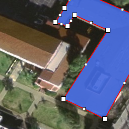
The Create and Edit sample illustrates how to create vector shapes on the map or modify existing ones via (freehand) map drawing. LuciadRIA supports points, polylines, polygons, circles, ellipses, circular arcs, elliptical arcs, arc bands, geo buffers and extruded shapes.
There are 2 themes in this sample:
- The "Default" theme: This theme demonstrates the out-of-the-box editing capabilities of LuciadRIA.
- The "Custom" theme: This theme demonstrates how you can customize editing and creation in LuciadRIA.
Functionality in both themes
Select an object to start editing it.
When editing the shape, you can drag the entire shape or move individual vertices by moving the handles. To insert vertices in a polyline, polygon or geo buffer, select the small handle in the middle of the line segment. To delete vertices in a polyline, polygon or geo buffer, press down and hold one editing handles of the shape's points. You can also hold down the Ctrl button, and click on a point's handle to delete it. To finish the editing, click on the map outside the shape.
When editing an extruded shape, a panel opens that shows the shape's minimum and maximum height. This panel is synchronized with edits you do on the map.
You can undo and redo shape edits by pressing the undo/redo buttons at the bottom of the page. Alternatively, you can press CTRL+Z and CTRL+Y to undo and redo shape edits. On Mac machines, you can also use CMD+Z to undo and CMD+SHIFT+Z to redo.
Default theme
Click one of the buttons in the toolbar at the bottom to start creating a new shape. You can create and edit the following shapes: a point, polyline, polygon, circle by 3 points, circle by center point, ellipse, circular arc by 3 points, circular arc by center point, circular arc by bulge, elliptical arc, arc band, geo buffer, as well as quadratic and cubic Bézier curves. To finish creating the object, click on the map outside the shape. For polylines, polygons, and geo buffers, double-click to finish.
While editing or creating shapes, you can revert back to the initial state by pressing the Escape key. If you already are in the initial state, pressing the Escape key will stop the edit or creation process. Alternatively, you can use the new buttons at the bottom when working on a touch-screen device. The left-most button will bring you back in the initial state, the selection button will stop the edit or creation process.
For polylines and polygons you can drag the mouse over the map for freehand drawing. After releasing the mouse, you can continue freehand drawing if you start to drag in the vicinity of the point where you finished.
Right-click on an object to show a context menu that allows you to:
- Edit the shape (similar to selecting the object)
- Delete the object
- Create a geo buffer based on the shape (for polylines and polygons)
- Create an extruded shape based on the shape (for all line and area shapes)
The features you create and edit are stored on the server. A
CustomJSONCodec
is used to exchange the features with a server. This codec encodes shapes as GeoJSON except for the shapes that
are not covered by the GeoJSON standard. For these shapes the
CustomJSONCodec
defines a custom encoding and decoding mechanism.
Custom theme
The custom theme shows some examples of how you can customize creation and editing in LuciadRIA. It shows the following customizations:
- 3D polyline (3D map only). Click on this line to edit it. You can change the height of each point individually by dragging the point that's floating in mid-air. The 3D polyline is also projected on terrain. Editing the projected line works just like the default 2D polyline editing behavior. You can move points, insert points and delete points on the line that's projected on terrain. You can also move the entire polyline by dragging the projected line.
- Star. Click on the star shape to edit it. You can only move the entire polygon, and not its individual points.
- Trajectory. Click on the "Trajectory" line to edit it. The start and end points of the line are always fixed. These represent the departure and arrival of a plane. You can not move the entire trajectory, and you can only edit intermediate points. You can create a trajectory from the toolbar at the bottom.
- Boundary. Click on the "boundary" shape to edit it. You can only edit individual points. Moving the entire shape is not allowed.
- Arrow. Click on the arrow shape to edit it. This arrow shape is not available out-of-the-box in the LuciadRIA API. This is a polygon that is edited as if it is an arrow. Drag the start and end points of the arrow to move them. The arrow can also be moved in its entirety. Dragging the corner of the tip of the arrow, changes its width. By holding SHIFT while changing the arrow width, the width snaps to multiple of 100. You also see helper lines and a label when changing the width. The arrow width is constrained to a minimum and maximum. You can create a new arrow shape from the toolbar at the bottom.
Symbology Encoding
This sample demonstrates Symbology Encoding in LuciadRIA. The sample loads a number of layers that are each styled using a Symbology Encoding definition.
It is possible to modify the Symbology Encoding definition for a layer and re-apply the styling information on the layer. By selecting a layer in the layer control, the corresponding style file is displayed in the code editor next to the map. When you are done making modifications, you can click the "Apply Style" button, or type Ctrl-Enter (⌘-Enter on Mac) to apply the style on the corresponding layer.
Note that the Symbology Encoding specification does not allow you to specify a different style for selected
features. To be able to differentiate between selected objects, the generated painter is equipped with default
selection behavior. See
luciad/view/feature/FeaturePainterUtil.addSelection() and
Use different styling for selected features for more information about selection styling.
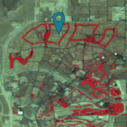
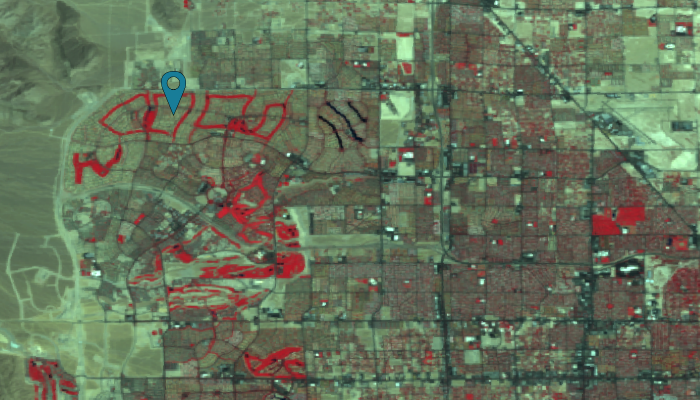
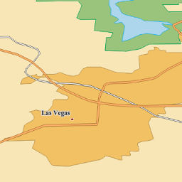
Multispectral Analysis
This sample shows two multi-spectral rasters of Las Vegas on top of each-other. The two datasets are from 2000 and 2003, and the sample allows you to instantly compare the two using a slider.
The raster data is served over WMS by a LuciadFusion server. The data is not pre-processed. The selected bands are sent to the WMS server using SLD.
Usage
- Use band selection to see an individual band in grey-scale.
- Use combinations to see interesting combinations of bands in color. Explanation of the selected combination is displayed on the right.
- Use the cross-fade slider to instantly see the difference between the data from 2000 and 2003.
- Select the blue pins: each show a balloon with something interesting at that location.
Details
The band selection is passed to the WMS server using the
SLD_BODY
parameter of the WMS request. It contains an SE
<RasterSymbolizer>
tag with SE
<ChannelSelection>
.
See
WMSTileSetModel
.
sldBody
and
WMSImageModel
.
sldBody
.
The cross-fade slider makes use of the
RasterTileSetLayer
.
rasterStyle
functionality.
Data Formats
This sample shows how to load and visualize data from the various data formats and web services supported by LuciadRIA. Support is included for GeoJson, GML, KML, OGC 3D Tiles, OGC WFS, OGC WMS, OGC WMTS, LTS, Azure Maps, HERE Maps, Google Maps, HSPC and OpenStreetMap tile services.
Usage
- Use Example data to load some example data on the map.
- Use Open File to open a local file (GML, GeoJson) or remote URL (GML, GeoJson, KML).
- Use Connect to service to connect to geospatial mapping services, such as Azure, HERE, Google, OGC services, ...
- Drag and drop GML or GeoJson files on the map.
Supported formats
Each format has a sample snippet file on how to load the specific data
format. See the files named
*DataLoader.js
.
GeoJson
Use a
GeoJsonCodec
in your
Store
.
Use a
FeaturePainter
to style your data using properties in the GeoJson file.
GML
GML 3.2 data, that adheres to the Simple Feature profile (SF-0).
Use a
GMLCodec
in your
Store
.
Use a
FeaturePainter
to style your data using properties in the GML file.
KML
OGC KML 2.2 data
Use a
KMLModel
with a
KMLLayer
.
- Features: Placemarks (Points, LineString, LinearRing, Polygon, MultiGeometry), Network Links (links to other KML files), Ground Overlays (images draped on terrain)
- Styles: LineStyle, PolyStyle, IconStyle (except color modulation), LabelStyle
- Other: balloons with static html, labels
- KMZ-files, which are zipped KML-files. Only the top level KML file in the KMZ and its image resources will be processed.
- Cross-Origin requests that do not contain an "Access-Control-Allow-Origin" header in the response can not be loaded.
- Styles have to be defined in the KML file itself, they can not be referenced externally.
- Screen Overlay features and Photo Overlay features are not supported.
- No support for KML schemas or extended data.
WFS
Use a
WFSFeatureStore
with the appropriate codec (
GeoJsonCodec
,
GMLCodec
or a custom codec).
Use a
FeaturePainter
to style your data using properties in the WFS response.
When using a WFS server, you can optionally specify an OGC filter as
your layer
query
that is passed along in the WFS request.
WFS data is automatically loading using
LoadSpatially
, but you can override it to
LoadEverything
.
WFS data can only be loaded if the WFS Server allows cross domain
requests.
For more information about setting up CORS for OGC WFS web services in
LuciadFusion, see
Using WFS in a Rich Internet Application (RIA).
This sample uses
https://sampleservices.luciad.com/wfs
as WSF service, which runs on a LuciadFusion server. This service is for
demonstration purposes only. You can use this service only for simple
tests and demonstrations. You should not rely on this service in any
way.
WMS
With the Tiled option you can choose whether to retrieve the data as a collection of tiles, or as a single image.
-
Tiled WMS is typically faster, but may have less visual quality
because images can be rescaled.
Use aWMSTileSetModelwithWMSTileSetLayer. -
Non-tiled WMS will have better visual quality, but a whole new image
for the entire screen has to be loaded each time.
Use aWMSImageModelwithWMSImageLayer.
Non-tiled WMS is not yet supported on a RIAMap.
This sample has a controller (
FeatureInfoController
) that will highlight a WMS feature on mouse over, and will shows its
properties in a balloon on select.
This sample uses
https://sampleservices.luciad.com/wms
as WMS service, which runs on a LuciadFusion server. This service is for
demonstration purposes only. You can use this service only for simple
tests and demonstrations. You should not rely on this service in any
way.
WMTS
See the sample code
WMTSTileSetModel
, in combination with
RasterTileSetLayer
.
This sample uses
https://sampleservices.luciad.com/wmts
as WMTS service, which runs on a LuciadFusion server. This service is
for demonstration purposes only. You can use this service only for
simple tests and demonstrations. You should not rely on this service in
any way.
Azure Maps
Use
AzureMapsTileSetModel
with
RasterTileSetLayer
.
HERE Maps
Use
HereMapsTileSetModel
with
RasterTileSetLayer
.
Google Maps
Use
GoogleMapsTileSetModel
with
RasterTileSetLayer
.
LuciadFusion
Use
FusionTileSetModel
with
RasterTileSetLayer
.
You can load imagery data as well as elevation data.
Elevation data has no effect in a 2D map.
This sample uses
https://sampleservices.luciad.com/lts
as LuciadFusion service, which runs on a LuciadFusion server. This
service is for demonstration purposes only. You can use this service
only for simple tests and demonstrations. You should not rely on this
service in any way.
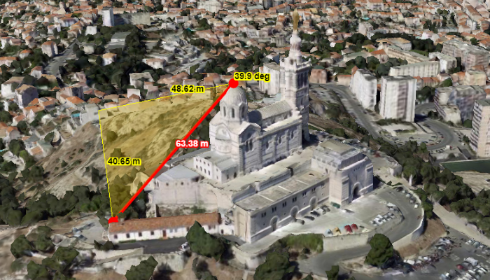
OGC 3D Tiles
Use
OGC3DTilesModel
with
Tileset3DLayer
.
You can load 3D tiled mesh data (In B3DM/GLB/glTF format) as well as Point Cloud
data (In PNTS format). The Marseille 3D mesh data used in this sample
has been created by Airbus with Airbus Street Factory.
Sometimes data density can be lower or higher than reported. Do not
hesitate to manipulate the quality factor to find the right balance
between precision and performance.
Google 3D Tiles
Use
OGC3DTilesModel
with
Tileset3DLayer
.
You can load Google 3D Tiles mesh data (in the GLB format) if you have a
valid Google API key.
Google 3D Tiles is supported on a 3D map only.
The resolution of the tiles received through the Google Map Tiles API may
provide the tiles at a lower resolution than what you can experience on
Google products (like Google Earth).
This sample uses
https://sampleservices.luciad.com/ogc/3dtiles
as OGC 3D Tiles service, which runs on a LuciadFusion server. This
service is for demonstration purposes only. You can use this service
only for simple tests and demonstrations. You should not rely on this
service in any way.
Hexagon Smart Point Cloud (HSPC)
Use
HSPCTilesModel
with
Tileset3DLayer
.
You can load point cloud data in the HSPC format with this API.
The default quality factor might not be perfect for every dataset. Do
not hesitate to manipulate the quality factor to find the right balance
between precision and performance.
OpenStreetMap (OSM) tile services
Use
UrlTileSetModel
with
RasterTileSetLayer
.
You can load imagery from OSM tile services with this API.
KML
This sample shows how to load KML data with Network Links and Ground Overlay features, and how to create a KML content tree user interface showing the hierarchical structure of KML data.
When you use KMLModel with KMLLayer then the underlying KMLCodec
decodes KML data and returns a Cursor of KMLPlacemarkFeature's only,
that are automatically visualized on a map.
KMLNetworkLinkFeature's and KMLGroundOverlay's have to be visualized differently.
KMLCodec emits the KMLNetworkLink event and the KMLGroundOverlay event
when these features are encountered in KML data. A custom event handler can consume these events by creating
a new KML layer for KMLNetworkLink and a new raster layer for KMLGroundOverlayFeature.
For more information please consult the KML API documentation and
the how-to article on visualization of KML data.
At the end of the decoding process, the codec emits a single KMLTree event that reports
the whole structure of KML data starting with the topmost KMLDocumentFeature, which is a container
feature that includes all KML feature types.
The sample builds the KML content tree user interface based on the emitted KMLTree and
automates creation of new layers for network links and ground overlays.
Instructions:
-
Use the fold icon to expand or collapse a KML container item.
The initial fold state of KML containers depends on KML
openelement. -
Click on the visibility icon to control the visibility of features.
The initial visibility of KML features depends on KML
visibilityelement. When the container's visibility is changed then the new visibility is propagated to all children. - Double-click on an item to performs an animated pan to the feature or a collection of features the item represents.
-
When a KML Network Link feature is defined with the
refreshModeequal toonIntervalthen the created KML layer refreshes its data every n seconds as specified initially in KMLrefreshIntervalelement. In such cases yuu can change the refresh interval using teh Refresh button. - When data is loaded a busy icon show up for a KML layer item, that represents the root layer or a layer created for a network link.
You can drag and drop a KML or a KMZ file on the map. KMZ-files, which are zipped KML-files. Only the top level KML file in the KMZ and its image resources will be processed.
The sample code is written in TypeScript with JSX. The user interface is built using the React library.
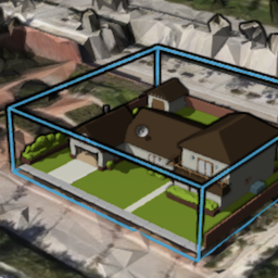
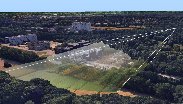
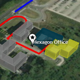
Geolocate OGC 3D Tiles
This sample shows you how to geolocate an OGC 3D Tiles dataset on the
globe. The prerequisite for this is that the sample dataset is not
already georeferenced. In the case of an OGC 3D Tiles, this means that
its metadata does not use the
Region
element, but instead a
Box
without a root level transform.
When an OGC 3D Tiles dataset is not georeferenced, its reference will be "LUCIAD:XYZ", which is a cartesian reference that does not contain geospatial information. The "LUCIAD:XYZ" reference does however say something about its axes: All axes are expressed in meters, and are pointing in specific directions:
- X-axis: East
- Y-axis: North
- Z-axis: Up
GeoLocateController
Internally, the
GeoLocateController
creates an
Affine3DTransformation
, which is a transformation that can convert the "LUCIAD:XYZ" reference
into a geospatial reference "EPSG:4978", an earth-centered, earth-fixed
geocentric reference.
Usage
- Click and drag the building icon onto the map. This will generate a new layer at the position of the mouse.
- When active, you can drag around the building by hovering over it and dragging the base plane around.
- When active, drag around the outer circle of the building to change its orientation.
- To move the building up and down, look at it from its side, and drag the vertical controls up and down.
- To slice the building, or to scale the terrain displacement, click on the Slice button (or press space) and drag the corresponding handles.
- Click on the fitting buttons in the corner of the map to move the camera to convenient geolocating angles.
- Press CTRL+Z and CTRL+Y to undo and redo changes to the geolocation. On Mac machines, you can also use CMD+Z to undo and CMD+SHIFT+Z to redo.
Data
Background data
There are two datasets you can choose from as background data in this sample.
-
By default, the sample works with The Marseille 3D mesh data, created
by Airbus with Airbus Street Factory and hosted by our LuciadFusion
server on
https://sampleservices.luciad.com/. -
You can also use Google 3D tiles as background data. To accomplish
that, provide your own Google API key in the URL of the sample as
&googleAPIKey=...YOUR_API_KEY...
Houses
The non-geospatial dataset of the buildings were created by Somnit and
ztrztr on
http://www.sketchfab.com and also hosted by our
LuciadFusion server on https://sampleservices.luciad.com/.
You can use these services only for simple tests and demonstrations. You
should not rely on either of them in any way.
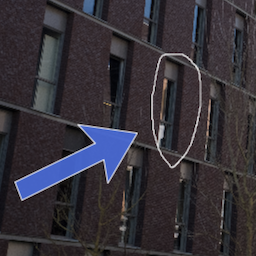
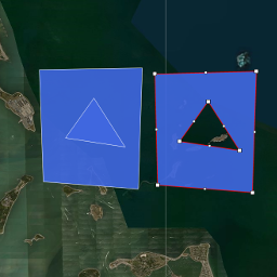
Image viewer
This sample shows how to visualize non-georeferenced images into a CRS:1-referenced map.
To view different images in the sample, simply drag and drop images from your desktop to the application. This will replace the existing image and load the image. Images are limited to the jpg, jpeg and png formats.
Navigation also works as it would on a regular georeferenced map. You can pan, zoom and rotate the map to see your image from different angles and zoom-levels.
The map you are seeing is projected in the CRS:1 reference. This reference is a special projection that works in pixel-space. In the CRS:1 reference, each world unit is one pixel in size.
This sample also demonstrates how you can annotate these images. Click on one of the buttons in the toolbar to draw a shape on top of the image. You can undo and redo shape edits by using the undo/redo buttons in the toolbar, or by pressing CTRL+Z / CTRL+Y. On Mac machines, you can also use CMD+Z to undo and CMD+SHIFT+Z to redo.
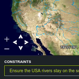
Navigation
This example shows how you can use the
map.mapNavigator
to change the center position and the scale of the map. It also shows how you can limit navigation by setting
a navigation constraint on the map.
Press the zoom and pan buttons on the map to perform an animated zoom and pan.
Use the dropdown to set a rectangle on the map beyond which you cannot navigate the map. This is useful to limit the map to certain areas.
The river layer is a WMS layer served by LuciadFusion.
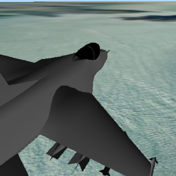
Camera
This sample illustrates how to use the Camera API using multiple custom controllers.
You can switch between the three controllers using the buttons at the bottom of the map.
On a mobile browser, the First Person controller is not available.
The First Person Camera Controller allows the control of the camera and modify its position using a predefined keymap to move and the mouse to change the camera's yaw and pitch. A guide image is displayed in the bottom right corner to show the keymap.
The Orbit controller consists of a camera orbiting around an F16 plane, keeping that point of interest in the center
of the view. This controller uses the
Animation
and
AnimationManager
API.
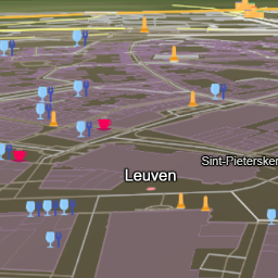
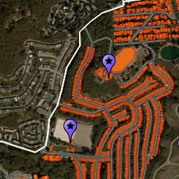
Smart Data Loading
This sample demonstrates how to handle large vector data sets by organizing that data according to multiple scale levels and configuring a loading strategy. This is illustrated by a number of Feature Layers that visualize large OpenStreetMap datasets: places, roads, buildings, and points of interest in Belgium.
A
QueryProvider
lets you define what kind of data should be presented at different scales. For example, at a large scale you only
want to show highways, while at a smaller scale, you also want to see local roads. On a 2D map, different data
will be loaded depending on the scale you're looking at. In the sample this is combined with the
LoadSpatially
loading strategy, which only loads the data for the current view extent. If the
LoadEverything
loading strategy is used, all the data for that scale level would be loaded.
In 3D scenes the
LoadSpatially
loading strategy will load data for multiple scales: data on the horizon is visualized with a larger scale because
it is farther away from the camera. The sample illustrates this by loading and displaying only highways on the
horizon, while close to the camera also the local roads are loaded and shown. Consult the
LoadSpatially
JSDoc for more information on how the loading strategy uses the
QueryProvider
to achieve this.
The sample shows the total number of features that are loaded into the
WorkingSet
of all layers. This counter is updated when you navigate over the map, as new data is loaded when scale level
zones change.
Learn how to include large vector datasets. Use scale levels to control data download size and to style points, lines and polygons according to your business rules.
Complex Stroking
The Complex Stroking sample illustrates how to use the "Complex Stroke" API in LuciadRIA. This is a powerful API that allows you to stroke lines with complex patterns and add decorations at specific locations along the line. For example, you could draw a line with a sawtooth pattern and decorate it with arrows at the start and the end of the line.
When you open the sample, you will see various shapes and lines that are stroked using the Complex Stroke API. Every shape is labeled with an identifier. You can use this identifier to see how the shape is styled in the sample code.
You can select an object to start editing it. Notice how the patterns dynamically follow the shape while editing.
The Cookbook Theme is intended for developers. You can experiment with complex stroked line styles by changing sample snippets, or by creating new complex stroke styles and visualizing the results. You can also edit shapes to check how the complex stroke style is drawn over the vertices of a shape.
For more information, see A step-by-step guide to complex strokes.
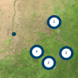
Clustering
The Clustering sample illustrates how to apply clustering to a data set containing a large number of armed events. Depending on the zoom level, the elements will be clustered appropriately, avoiding a cluttered view.
The sample contains a large number of armed events that took place in Africa. When a number of events are close together (in view-space), they become hard to distinguish. Therefore, a cluster is shown instead of the individual events.
It is also possible to compare the original model and the clustering transformed derivative by using the "ENABLE CLUSTERING" check box.
Creating a clustered data set through code is done by creating a
ClusteringTransformer
, and setting this transformer on a
FeatureLayer
.
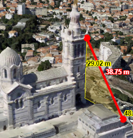
OGC 3D Tiles
This sample shows how to load 3D tiles with meshes and point cloud data on the map. It also shows you how to style meshes and point clouds with expressions, allow measurements on meshes and point clouds, add effects to your map, and drape shapes on top of meshes. The map supports both 3D and 2D projections.
Usage
- Click Marseille Railway Station dataset to load the point cloud data on the map.
- Use 3D ruler controller to measure distances, angles and surface of area.
- Hover over the Railway Station layer in the layer tree, and click on the three dots to access the layer settings.
- Use styling expressions for the Point Cloud layer to modify the size, color, and visibility of individual points.
- Use Quality slider for each layer individually to apply the level of detail multiplication factor for the geometric error that determines the how detailed tiles should be loaded.
- Use Effects and Light to play with different graphical effects on the map.
- Select the walking route (orange line) or some points of interest (icons) along the walking route to show a balloon with more information about the clicked item.
Features
3D data
Use
OGC3DTilesModel
with a
TileSet3DLayer
.
You can load 3D tileset data on 2D and 3D maps.
Note: The elevation data has no effect in a 2D map.
The 3D ruler controller displays various measurements: distance of 3D line segments, angles between points, orthogonal distances, heights over terrain, and area surface, depending on the selected measurement mode. To start a measurement tool, turn on the 3D ruler controller and click on the map in order to add new points for measurement. Each additional click adds a new segment to measure. You can change the measurement mode on the measurement panel.
The 3D ruler uses
RIAMap.getViewToMapTransformation
API with
LocationMode.CLOSEST_SURFACE
mode. This transformation object provides for the given view position a map point on the closest surface, that is
a 3D object represented by meshes, point cloud points, extrudes shapes, or terrain.
This transformation is used on 3D maps only.
The Effects and Lights tools show various graphic effects that can be applied on a 3D scene. In the effects panel you can change the camera focus depth, you can enhance depth perception by enabling eye-dome-lighting, and you can play with the color palette of the scenery. In the light panel you can enable sunlight with shadows and atmosphere lighting, ambient occlusion and fog effects.
Expression based styling
The
TileSet3DLayer
allows to set
PointCloudStyle
that defines the expression based styles for the point cloud data.
The are three types of expressions:
- colorExpression
property defines colors for point cloud point. By default colors are defined in the tile data. If no color is
defined, LuciadRIA paints them in white. You should use
ExpressionFactoryto define an expression that evaluates to a color value, e.g. based on attributes in the batch table section of the PNTS data. - visibilityExpression
property is a filter that determines point cloud data visibility. You should use
ExpressionFactoryto define an expression that evaluates to a boolean value. - scaleExpression
property controls point size. By default points are visualized as rectangles of size 3 on 3 pixels. You should
use
ExpressionFactoryto define an expression that evaluates to a number value, that is interpreted as scale factor. The scale factor of value 1 preserves the original size, a value greater than 1 enlarges points, and a value lesser than 1 makes points smaller.
The TileSet3DLayer that contains the 3D tiles with meshes is marked as a drape target using the
isDrapeTarget constructor parameter. This means that data can now be draped on this layer.
To drape the walking tour shape, it is styled with a ShapeStyle in which the drapeTarget
parameter is set to DrapeTarget.MESH.
Data
The Marseille 3D mesh data used in this sample was created by Airbus with Airbus Street Factory. The train station
lidar data was created by Flying-Cam for Altametris and SNCF Réseau. Both datasets are available as OGC 3D Tiles
services, hosted by our LuciadFusion server on
https://sampleservices.luciad.com/
. You can use these services only for simple tests and demonstrations. You should not rely on either of them in
any way.
OGC 3D Tiles Property Injection
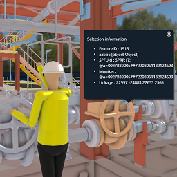
This sample demonstrates how to inject static or dynamic feature properties in a OGC 3D Tiles layer. It also demonstrates how to monitor changing feature information through selection and expression based styling on 3D data through OGC 3D Tiles.
The data
This sample shows a Smart Site dataset. The dataset is an industry plant CAD model, made available as Hexagon PPM "BINZ" data through Smart InterOp Publisher. It has been converted to OGC 3D Tiles through LuciadFusion. This process retains metadata information such as linkage, moniker, and featureID.
The OGC 3D Tiles data is then displayed using a TileSet3DLayer.
Selection
The layer has been made selectable, and uses the featureID to distinguish individual objects. When you click on an object, it is highlighted and a balloon is displayed, showing the properties of the selected object. The sample code also shows different ways of listening to selection events, and how to retrieve relevant data from the selected object.
Properties
The sample code adds two properties to the layer. The first property "PipeWithSensor" is a static property. Its default value is "0", indicating that no sensor is attached. The value gets updated once, for the piping right behind the operator in the startup view. It gets value "1", indicating that a temperature sensor is attached. The second property "PipeTemperature" is a dynamic property, meant to visualize the temperature of the pipe to which the sensor is attached. The temperature is updated every 200 milliseconds, and is used in a color expression. It lets the pipe change color as the temperature changes, and show possible overheating. When you select a part of the color-changing pipe, you will see that the temperature is also updated in the selection balloon.
Visual effects
This sample shows a number of visual effects that enhance the display of CAD data:
- Anti-aliasing (see
map.effects.antiAliasing): avoid aliasing effects on sharp CAD object edges. - Regular lighting (see
map.effects.light): enhances the 3D visualization. - Ambient occlusion (see
map.effects.ambientOcclusion): enhances realism by adding soft shadows. - Transparency (see
TileSet3DLayer.transparency): allows painting transparent objects. - Environment map (see
map.effects.environmentMap): allows showing a skybox and defining a reflection map that will be used when PBR materials are available on the model.
Navigation
An asset navigation controller has been integrated to facilitate navigation. You can use the default navigation keys to move your camera left, right, forward, backward, up (E) and down (A or Q), unrestricted by walls and floors. When navigating using your mouse, a gizmo is provided to visualize the anchor point for navigation, panning, or rotating action.
Extra tools
This sample includes additional tools available from the toolbar located at the top left of the screen:
-
The
Magnifiertool enables detailed inspection of the BIM models. When activated, it allows for close examination of specific areas without changing the camera position. Users can adjust the magnification factor by scrolling the mouse wheel while pressing the Shift button. Scrolling with the Control key pressed will resize the magnifier viewport. -
The
CrossSectiontool allows you to slice the map and display a cross-sectional view - a Cartesian map on which measurements can be performed. -
The
Tourtool manages and animates tour paths. With this tool, you can create, edit, and animate geospatial tours, simulating journeys along custom paths. It also allows you to record these tours. The Tour tool provides the features to control duration, speed, and looping of animations.
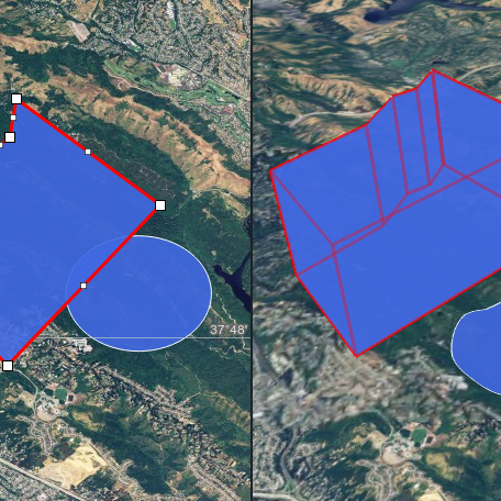
Dual Map Sample
This sample illustrates the power of the Model-View separation in LuciadRIA by showing two synchronized views based on the same data. It also shows you how you change map projection at runtime. It also shows you how you can load and use references that are not included by default in LuciadRIA.
There is a 2D map on the left and a 3D map on the right. Selection is automatically synchronized between the two maps. You can edit shapes on the left map, and the changes will be applied to the right map.
The toolbar on both maps allows you to create various shapes. Creating new shapes is similar to the "Create and Edit" sample.
The context menu allows you to extrude an existing flat shape, turning it into a 3D volume.
The reference picker allows you to change a map's projection.
You can undo and redo shape edits and selection changes by pressing CTRL+Z and CTRL+Y. On Mac machines, you can also use CMD+Z to undo and CMD+SHIFT+Z to redo. Undo/redo actions are shared across both maps.
Labeling
This sample demonstrates how to paint decluttered labels for points, polylines and polygons. The sample uses three layers with vector data from the US. Each of these layers uses a separate painter that defines the specific styling that should be applied to the vector data.
To paint labels, every painter overrides the
FeaturePainter.paintLabel()
method and uses the
LabelCanvas
to paint labels. Depending on the properties of a feature, different styling for both the label and its shape is
applied.
The state labels are repositioned whenever a previous label location becomes invisible in the current view. You
can deactivate this behavior for in-path labeling by using
InPathLabelStyle
with the
inView
property set to false. In this case, the labels are placed in the center of the shape. They are not redrawn if a
label threatens to go off-screen. Additionally labels for the River layer are repeated along polyline geometries
using
OnPathLabelStyle
.
In addition, the state labels are drawn with the
InPathLabelStyle#restrictToBounds
style property. The flag indicates if the label should be painted outside of the bounds of its painted shape or
not.
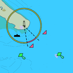
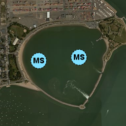
ECDIS
This sample shows an ECDIS layer served over WMS by a LuciadFusion server. The user interface allows you to customize the ECDIS visualization. The visualization parameters are sent to the WMS server using SLD.
See
WMSTileSetModel
.
sldBody
and
WMSImageModel
.
sldBody
.
For instance, you can change the color scheme by clicking on the Day , Dusk or Night buttons.
The sample also illustrates the use of WMS GetFeatureInfo requests to retrieve feature information for selected features. Select the corresponding checkbox to retrieve and show feature information for a clicked location on the map.
ECDIS S-57 ENC dataset provided by NOAA . For demo purpose only.
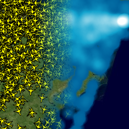
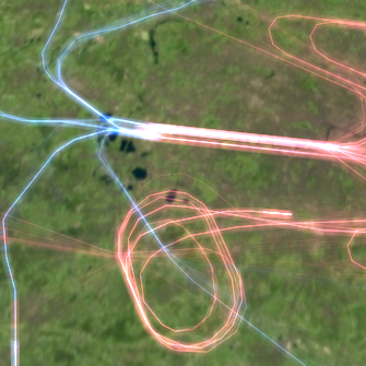
Tracks
The Track Display sample illustrates how to display 5000 moving tracks received via a web-socket. Density analysis can be applied in a static way on the trajectories or dynamically on the moving tracks.
There are two datasets:
- Tracks : 5000 moving tracks, pushed from a server over a web-socket.
- Routes : the routes each of these tracks is moving over.
You can also enable static density , showing density over the routes.
For more information about pushing changes over web sockets, see WebSocketStoreDecorator.
For more information on density painting, see
FeaturePainter.density
.
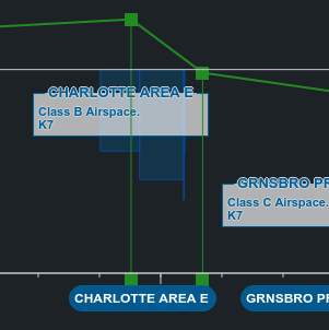
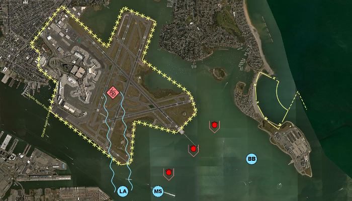
Vertical View
This sample demonstrates how a map with a Cartesian reference can be used to create a vertical view. The map displays airspaces and aircraft trajectories, while the vertical view shows which airspaces are intersected by the selected trajectory. It also helps identify the locations and altitudes where the aircraft enters and exits those airspaces.
The trajectories are represented by a green polyline in both the regular map and the vertical view. The airspaces are represented by polygons. The airspaces have a minimum and maximum height property. Those heights represent the lower and upper altitude bounds of the airspace.
When you select a trajectory, the vertical view updates to show that specific track. The X-axis represents the distance along the trajectory (0 meter meaning the start of the track) and the Y-axis represents the altitude in FL (flight levels). This allows you to determine the aircraft’s height at any point along its path.
The vertical view also shows the airspaces whose boundaries are crossed by the aircraft, represented as rectangles. The lower and upper height of the rectangle (the Y-coordinates) are determined by the minimum and maximum altitude of the airspace. The X-coordinates indicate where the trajectory enters and exits the airspace. When the aircraft passes below or above an airspace, the polyline in the vertical view runs below or above the corresponding rectangle. When the aircraft enters the airspace, the polyline passes through the corresponding rectangle. Airspaces not intersected by the aircraft are not shown in the vertical view.
Note that the trajectory and airspace layers in the vertical share the same models as their layers on
the main map. The conversion from a feature contained in the model to the shape displayed in the
vertical view is handled by a ShapeProvider on the FeatureLayer (see the
AirspaceShapeProvider and TrajectoryShapeProvider).
For more information about the
ShapeProvider, see the
non-map view documentation.
Because the model is shared between the main map and the vertical view, any updates to the trajectory on the map (right-click → Edit, then double-click to confirm) are immediately reflected in the vertical view.
The layout of the vertical view is created by the
@luciad/ria-toolbox-map-borders toolbox, which constructs the main Cartesian map
together with the bottom and left border maps configured as axes.
For more information on how to use the Map Borders toolbox, see the
"How to draw a map with borders" article.
Navigation is supported in the main map, the vertical view, and the border maps. The border maps allow zooming along a single axis without changing the scale of the other axis (non-uniform zooming). Use the mouse wheel on a border to zoom in or out along that axis. Using the mouse wheel inside the Cartesian view scales both axes simultaneously.
Note that airspaces and trajectory control points are drawn on border maps,
using dedicated FeaturePainter logic implemented by
AirspaceBorderPainter and TrajectoryBorderPainter.
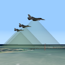
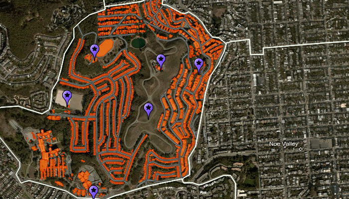
3D Icons
The 3D icons sample illustrates how to display and style 3D icons (meshes).
The sample shows the San Francisco area brought to life by the use of 3D icons. When you start the sample you see an F35 aircraft with a transparent cockpit and a billboard showing an advertisement ad for HxDR on a carrier aircraft's deck. In the background the Alcatraz prison is visible. When you turn around, you see the Golden Gate Bridge in the distance. You can also see military aircraft patrolling the airspace around the carrier.
All icons are selectable. When you select one, you can inspect it in more detail in an overlay asset viewer. The asset viewer loads the selected icon in a Cartesian view with a perspective camera. After loading, the icon is centered in the view, slowly rotating automatically by means of an orbit controller. You can control the rotation and zoom in or out to inspect the icon from all sides.
These 3D models are provided for sample purposes only and should not be used in an application that is violating the 3D Warehouse General Model License Agreement . 3D Warehouse General Model License Agreement provides that “You may not, and you may not permit anyone else to […] aggregate any content (including Models) obtained from 3D Warehouse for redistribution, or use or distribute any content obtained from 3D Warehouse in a mapping or geographic application or service, except as expressly authorized under this License Agreement.”
This sample also demonstrates some easily configurable simple 3D icons. A dome encases Alcatraz Island, while aircraft circle it. The aircraft have a field of view which is visualized by a cone.
There are a number of ways to define a 3D icon. You can
- specify a URL to a GLTF file.
-
create a simple configurable 3D icon using
Simple3DMeshFactory. -
create a 3D icon at the triangle level with
MeshFactory.
FeaturePainter
in combination with a
Icon3DStyle.
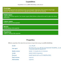
LuciadRIA device support
The device support sample gives you an overview of supported features, unsupported features and limitations of a RIAMap due to the capabilities of your device and browser.
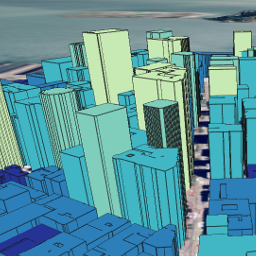
Extruded Shapes
The Extruded Shapes sample illustrates how to use extruded shapes to visualize a city landscape. The buildings are styled according to their height, using a thematic color range.
See
ExtrudedShape
on how to create extrusions based on a base shape and a minimum and maximum height.
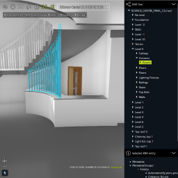
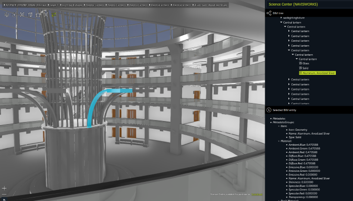
BIM Viewer sample
This sample can be used to visualize all converted supported BIM formats (Binz, IFC, Revit, Navisworks) datasets together with their original metadata. Their geometry needs to be converted to and served as OGC 3D Tiles. Their feature information needs to be converted to and served as GeoJSON or WFS service. To convert and serve the data, you can use LuciadFusion.
The data
- Navisworks: Science Center, available for purchase as Revit file on TurboSquid, and converted with Autodesk Navisworks.
- Revit: Commercial Building, available for purchase on TurboSquid.
- IFC: Medical Clinic, made available as a collection of IFC files by buildingSmart International: BSI (2020) "Medical-Dental Test Files," buildingSMART International.
- Binz: Industry Plant, made available as Hexagon PPM "BINZ" data through Smart InterOp Publisher.
All these datasets have been geolocated and converted to OGC 3D Tiles and GeoJSON through LuciadFusion. This process retains metadata information, as well as the tree-structure of the original BIM files.
The OGC 3D Tiles data is then displayed using a TileSet3DLayer.
The GeoJSON data is queried via an UrlStore, the tree structure of the BIM files is shown in the
top-right "BIM Tree" panel.
The sample also allows loading your own converted BIM datasets, with or without feature information. You can do this by choosing "Add a custom dataset ..." in the data selector dropdown.
Selection
The layer has been made selectable, and uses the featureID to distinguish individual objects. When you click on an object, it is highlighted and its properties are shown in the bottom-right "Selected BIM entity" panel. The sample code also shows different ways of listening to selection events, and how to retrieve relevant data from the selected object. Note that you can easily distinguish between currently visible and occluded selected items. The occluded ones only get a highlighted outline.
Navigation
An asset navigation controller has been added to ease navigation. You can use the default navigation keys to move your camera left, right, forward, backward, up (E) and down (A or Q) without the restriction of walls and floors. When navigating using your mouse, you get a gizmo-controller to help you see the anchor point of navigation as well as arrows when you are panning and circles when you are rotating.
Note that for custom datasets, the initial camera position is chosen to be in the center of the bounding box of the model. Although this might put the camera at an odd position, inside a wall for example, it is the only way to make the navigation controller work. You can easily get yourself in a better position by using the navigation keys. You can also fit to a selection to get a potentially better camera position.
Properties
Properties of features are queried on-demand from the GeoJSON dataset. The sample also contains the code that would be needed to query a WFS service with the feature information.
Note that properties for custom datasets can only be queried if you provided a Features URL when adding the dataset.
Visual effects
This sample shows a number of visual effects that enhance the display of CAD data:
- Anti-aliasing (see
map.effects.antiAliasing): avoid aliasing effects on sharp CAD object edges. - Regular lighting (see
map.effects.light): enhances the 3D visualization. - Ambient occlusion (see
map.effects.ambientOcclusion): enhances realism by adding soft shadows. - Environment map (see
map.effects.environmentMap): allows showing a skybox and defining a reflection map that will be used when PBR materials are available on the model.
Balloons
The Balloon sample illustrates the use of balloon widgets on the map. The contents of a balloon can be specified with a string or with valid HTML.
Add balloons to the map by using the
showBalloon()
method. Remove them from the map by calling
hideBalloon()
.
The contents of a balloon can be specified with a string or with valid HTML.
Balloons can be anchored to an object (for instance, a Feature from the model which is visualized by a FeatureLayer). Updates of the location of the feature cause the balloon to update as well.
Balloons are styled in the samples/common/ui/sample-common-style.css style-sheet. These styles may be
replaced with your own custom styles.
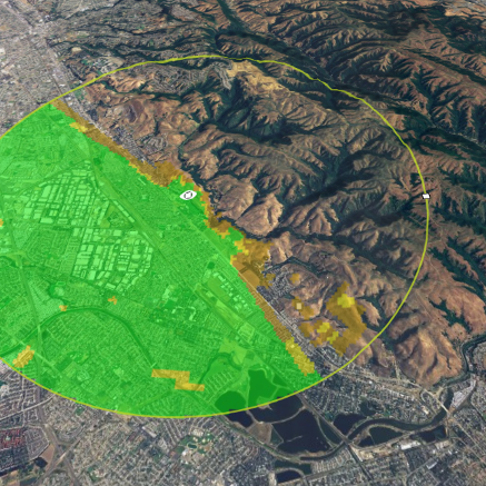
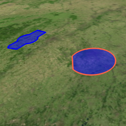
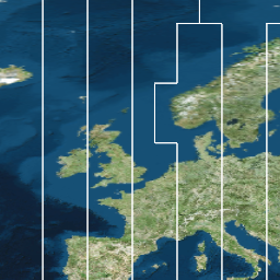
Terrain Services
The terrain services sample illustrates how LuciadRIA supports streaming and visualization of worldwide high-resolution terrain. Imagery is draped over the terrain for a realistic 3D experience.
There are two layers:
- An Elevation layer, which is visualized as 3D terrain
- A Aerial imagery layer with detailed imagery in San Francisco and Los Angeles
See
FusionTileSetModel
and
RasterTileSetLayer
on how to add terrain data to your map.
The height read-out makes use of the height service if it is available. If not, height data of the model is used.
If the LOS service is enabled, you have access to two additional layers:
- An LOS circle layer, which highlights the radius where the LOS is calculated
- A LOS data layer, which shows the output of the LOS service
The LOS service provides a visibility calculation from a person's point of view. The calculation is based on a digital terrain model. The result of the calculation provides information on what may be visible when looking around from the given location. Each color represents the minimum height range a person or object needs to be in to be visible. Actual values and colors used by the service to interpret the result are available in a legend.
For more details on the height and LOS services, you can visit the official documentation here.
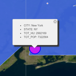
Selection and Filtering
This sample demonstrates various API features of selection and filtering in LuciadRIA. This includes:
-
Listening to the
onSelectionChangedevent on aFeatureLayer. - Styling non-selected and selected features using the same painter.
- Filtering of objects with a predicate function.
You can select an object by clicking on its visualized shape or on its label. Only objects in layers that are
selectable can be selected.
If a selected object does not pass the feature filter evaluation, it automatically gets deselected.
Use the slider to filter cities by population. The slider is a HTML5 form input control. The exact behavior depends on the browser. In some browsers, the values are updated continuously, while in others there will only be an update after the slider button has been released.
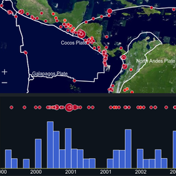
Timeline
This sample shows how to use a LuciadRIA RIAMap to display time-based data and expression-based styling.
Data
The sample shows an overview of world-wide earthquakes from 2000 to 2011, as well as the tectonic plates of the planet. Both are GML files that are styled and filtered using properties from the files.
The dot size indicates the earthquake's
magnitude
: larger dots for stronger quakes.
The dot color indicates the earthquake's
depth
: quakes near the surface are red, deeper quakes are yellow to blue.
The sample also shows a timeline with the earthquakes and a histogram.
The histogram shows the accumulated magnitudes of the visible earthquakes per month.
The sample offers playback functionality, activated by the corresponding button.
In playback mode, the styling dynamically changes based on the time of the earthquake and the time index indicated
by the vertical line in the timeline view. Only earthquakes that happened shortly before the indicated time index
are displayed.
Usage
You can navigate the timeline by zooming and panning.
The spatial map and the timeline are linked:
- The spatial map displays only earthquakes in the time range visible on the timeline.
- The timeline displays only earthquakes in the area visible on the map.
- Selection is synchronized between both views.
- The histogram updates automatically to reflect the visible earthquakes.
Details
The timeline is based on a LuciadRIA "non-georeferenced" map. It is a regular
RIAMap
to which you can add layers, but it doesn't have a spatial reference. Instead, it represents data over time.
Geometries can be defined directly in the time reference within your model, or generated dynamically
using a ShapeProvider that produces time-based shapes.
The timeline view layout is created using the
@luciad/ria-toolbox-map-borders toolbox, which renders the main Cartesian map
(the histogram) and the bottom border map displaying the time-based axis.
See TimeSlider for additional details.
The spatial map displays the earthquakes with a ParameterizedPointPainter instead of the regular
FeaturePainter.
It illustrates that you can not only achieve a similar visualization using expressions but also make use of fast
filtering, immediate density and dynamic styling.
See
EarthquakesParameterizedPointPainter
for details.
Advanced GIS Engine
Constructive Geometry
This sample illustrates the application of the operators union, intersection and difference to groups of shapes. All calculations are performed client side.
Constructive geometry operations can be applied by using the context menu. At least two shapes must be selected. To select multiple shapes, click on them while holding down the shift key.
To create new shapes use the toolbar buttons. To edit shapes right click on them and select 'edit'.
The constructive geometry operations are calculated using a
ConstructiveGeometry
instance which is created through a
ConstructiveGeometryFactory
.
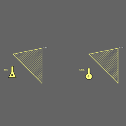
Defense Symbology
Military Symbology
A sample that demonstrates the modeling, visualization, editing and creation of military icons and tactical graphics, for the MS2525 and APP6 standards. See the Military symbology guide for more details.
The sample starts up with a few tactical graphics and icons already initialized on a map. Clicking on a feature
will display a panel containing some of its properties. Modifying the properties can be done in this panel. The
panel itself is part of sample. (Have a look at the
@luciad/ria-sample-milsym-common-ui/properties/SymbologyPropertiesPanel
module).
To create a new icon or graphic, type a symbol name in the creation panel on the top of the view. Selecting an item from that list will show you an instructions panel with a preview image of the symbol as well as some instructions on how to proceed with creation. Click on the map to draw your new military symbol. This panel is also part of sample. (Have a look at the symbology/CreationPanel module).
To edit an existing symbol, right-click the symbol and select edit. For devices that don't support right-click (such as touch-based devices), select a symbol and press "Edit Symbol" in the properties panel.
Not all modifiers that can be edited with the editing panel will change the visual presentation of the symbol. They only change the modifier of the object. This is for example the case for the "Country" modifier. This changes the attributes of the domain object, but does not change the visualization of the object. This is because the symbology standards, such as MS2525b, do not specify a change in visualization for all possible modifiers of the symbol.
This sample also demonstrates how to cluster military symbols. The following rules are applied:
- Units of different affiliation are not clustered together
- Units of different category are not clustered together. For example, ground units will not be clustered together with air units
- If a cluster contains several instances of the same military symbol, the symbol's icon will be used to represent the cluster, only bigger and with a label indicating the number of elements in the cluster.
- If a cluster contains different military symbols, a simple round icon with a label indicating the number of elements will be used.
- Sea Surface, Sea Subsurface and MineWarfare units will not be clustered
- A cluster must contain at least 2 military symbols.
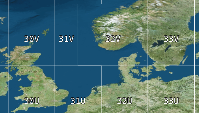
MGRS Grid
MGRS (Military Grid Reference System) is an alphanumeric multi-level, multi-reference grid used by NATO. The grid starts with 60 zones, plus the north and south pole area. As you zoom in, each zone is refined into 100.000m squares that are defined in a zone-specific reference system. These squares are then further refined up to the meter.
Using the panel on the right you can change the styling options of the grid. The results are applied instantly.
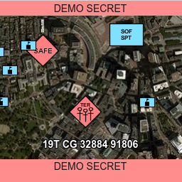
Military Symbols Overview
This sample shows all supported military symbols for the MS2525 and APP61 standards. The sample allows you to toggle between various parameters and standards, to see what effect they have on styling.
The layer tree shows you these layers:
- The Symbols layer displays the actual symbols.
- The Descriptions layer shows you in text the code of the symbol (including the SIDC modifiers), the name of the symbol and the code of the symbol without modifiers (base code).
- Only for tactical graphics: the Anchor Points layer shows you the points that were used to create the symbol.
Use the search bar to look for a specific symbol, either by name or by code. The auto-completion only allows you to search symbols that are visualized on the map.
When the sample runs in a WebGL environment, tactical graphics layers are pre-loaded using skeleton styling, a simplified styling without complex strokes or decorations. The pre-loaded skeletons allow you to start working on the layer (search for a symbol, select, change properties, edit) before the layer is fully loaded. To keep the layer responsive, the symbols are invalidated one by one, and redrawn in their full complexity using body styling. You can track the loading with a progress indicator in the layer tree.
1 We currently offer partial support for APP-6E. For this standard, only the icon symbols from the Cyberspace symbol sets are available. You can therefore only see APP-6E symbols when selecting the icons display mode, in the selection bar below the map.
COP Sample
The Common Operational Picture (COP) sample is a showcase of a real-world application built with LuciadRIA and LuciadLightspeed. It combines various capabilities of the two products to provide a COP view for the user.
To learn how to use the COP sample, see the COP user's guide.
The COP client connects to the COP services. A description of the COP services is available here .
Panoramic
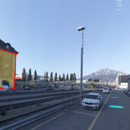
Panorama
This sample illustrates how to use LuciadRIA's Panorama API. A panorama is a photo with a very wide field-of-view, often even covering the full 360 degrees.
Click any panorama icon on the map or overview map to show the corresponding panorama. When you're inside a panorama, you can click the "Leave Panorama" button at the top of the screen to switch back to the 3D map. You can make 3D measurements both in and outside of panorama mode.
This sample can also be used to quickly inspect your own panoramic services. To do this, click on the button in the bottom bar and fill in the url to your service.
In the sample code, you'll find a number of controllers and animations you can re-use and adapt in your own projects. The usage of the actual RIA Panorama API can be found in view/PanoramaFeaturePainter.ts and LayerFactory.ts.
The default data in this sample is provided by Hexagon Digital Reality.
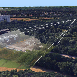
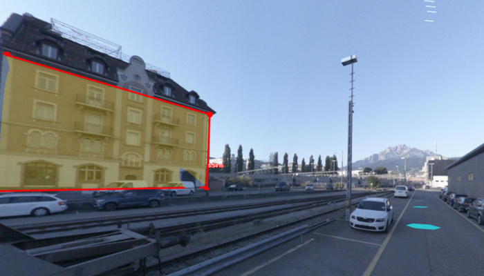
Video panorama
This sample illustrates how to use LuciadRIA's Panorama API for videos. Videos typically projected in this way are for example drone or security camera footage.
Use the video controls of the video panel on the left to control the video playback. The video is projected onto the map based on various metadata associated with each frame of the video.
The map's camera follows the drone by default. You can toggle this behavior with the camera lock button at the top.
For more information, see How to visualize panoramic video footage.