Rectification is the process that corrects the distortion introduced in aerial and satellite imagery, so that the images can be more accurately georeferenced. In general, rectification methods can be classified into parametric and non-parametric methods. Parametric rectification uses prior knowledge about the properties of the imaging sensor (plane or satellite trajectory, altitude, orientation) and the terrain elevation. Non-parametric rectification relies on manually defined tie points, relating image coordinates to known geographic locations using a mathematical function. It does not explicitly model the variations in terrain altitude.
The first part of this article presents non-parametric rectification. It is mathematically simpler, and therefore potentially less accurate. Section Transformations in a non-rectified grid reference starts by illustrating the chain of transformations used for mapping the pixels from an image to their corresponding geographical locations in more common geographical references. Section Transformations in a rectified grid reference continues with an explanation of the place of the rectification within this framework, and section Interfaces and classes used for rectification briefly describes the LuciadLightspeed classes involved. The second part of this article presents parametric rectification, also known as orthorectification. Section Parameters related to the imaging sensor introduces the camera parameters and section Including terrain information explains the usage of terrain elevation. Finally, the last part of the article shows how parametric and non-parametric rectification can be combined.
Non-parametric rectification
Transformations in a non-rectified grid reference
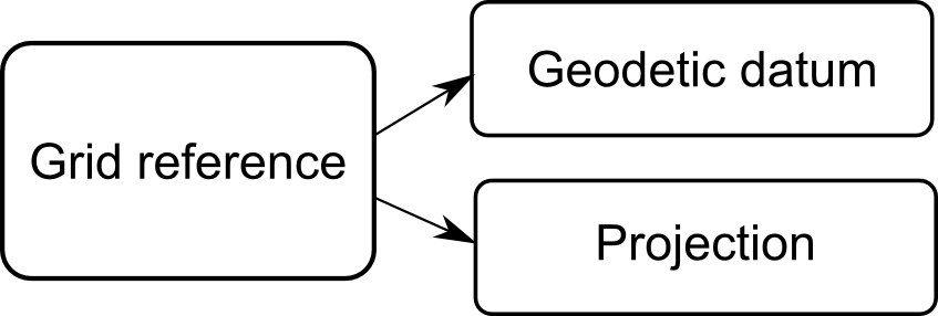
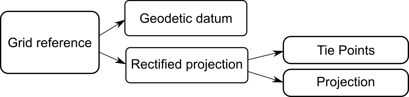
A grid reference system is composed of two main parts: a geodetic datum and a projection as shown in Figure 1, “A grid reference requires a datum and a projection”.
In general, to display an image in a geographical system, you need to define three distinct coordinate systems:
-
the image coordinate system, expressed in pixels
-
the grid (raster) coordinate system, usually expressed in meters
-
the geodetic coordinate system, expressed as longitude/latitude in a given geodetic datum
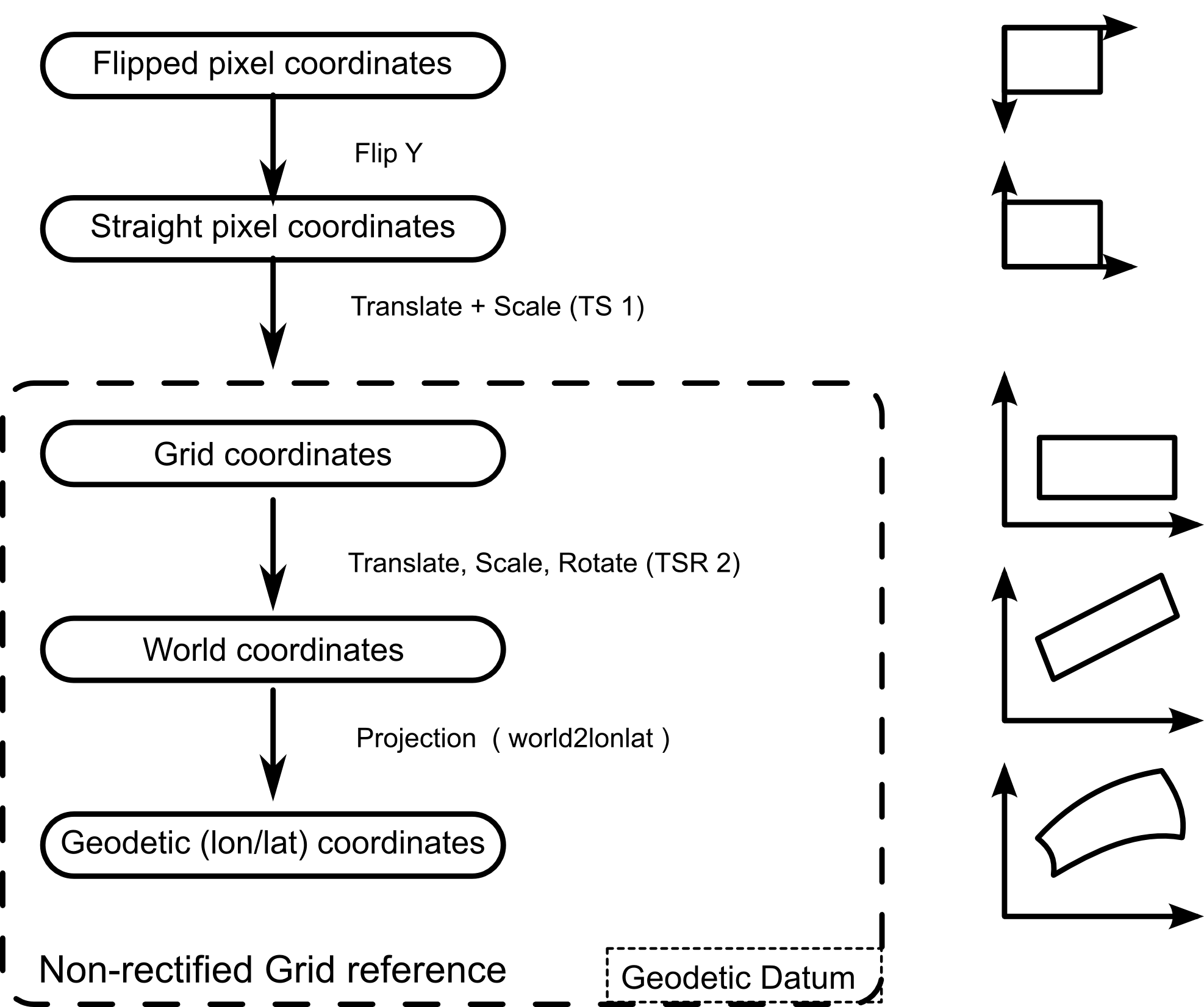
Apart from these three, other auxiliary systems may be used; see Figure 2, “Transformations from pixels to geodetic coordinates in a non-rectified grid”. For example, when an image is initially read from disk, it is in a flipped system — the origin of the image is in the upper-left corner with the Y axis pointing down, while in most Cartesian coordinate systems, the origin is considered to be the lower-left corner of the image with the Y axis pointing up (straight pixel coordinates).
In the grid reference system, the boundaries of the raster are assumed to be aligned with the axis of coordinates, so in order
to map a point from image coordinates to grid coordinates you only need to perform a translation and a scaling transformation
(TS 1). This transformation is performed transparently by the TLcdRaster class or by the equivalent implementation of the ILcdRaster interface.
From grid coordinates, a translation+scale+rotation operation (TSR 2) is applied to get to world coordinates, followed by
a projection that produces geodetic coordinates (world2lonlat). Geodetic coordinates can then be transformed to any other
reference system (for example, to the ILcdXYWorldReference of the map, during displaying).
Transformations in a rectified grid reference
Conceptually, the principle behind a rectified grid reference is identical to the non-rectified case. There are only a few practical differences, as shown in Figure 3, “Transformations from pixels to geodetic coordinates in a non-rectified grid”. The grid coordinates and the pixel coordinates are usually the same. After the initial translation+scale+rotation (TSR2) operation, non-rectified world coordinates are obtained which are passed through a rectifying function to obtain world coordinates. A normal projection is then applied to finally get geodetic coordinates.
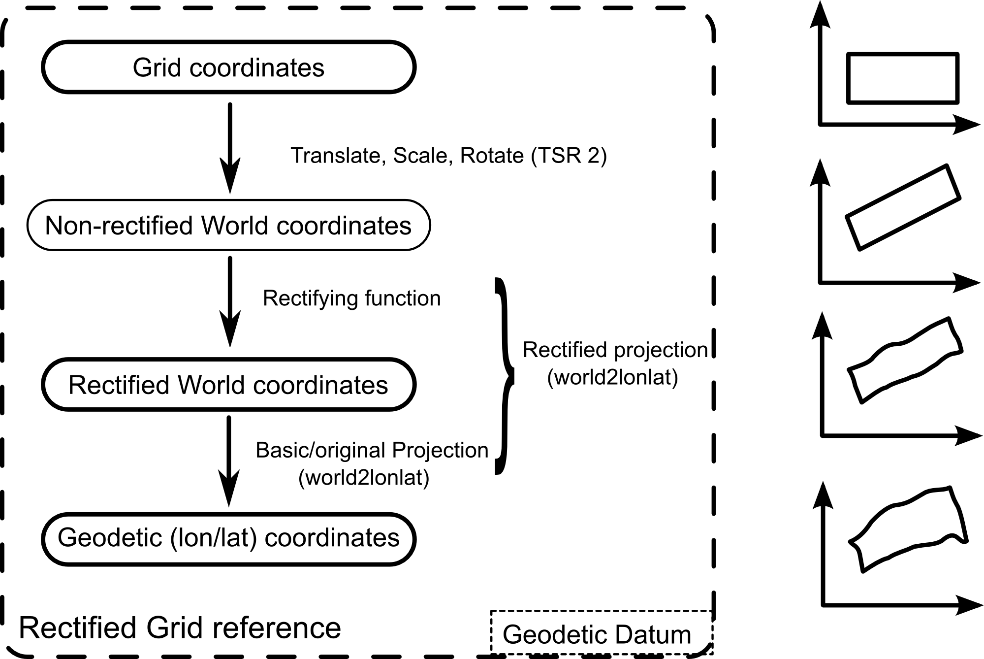
To keep the API consistent, the rectifying function and the projection step are grouped in a special type of projection — an
ILcdRectifiedProjection — which wraps the traditional projection. This allows for a rectified reference to be used just like any other grid reference.
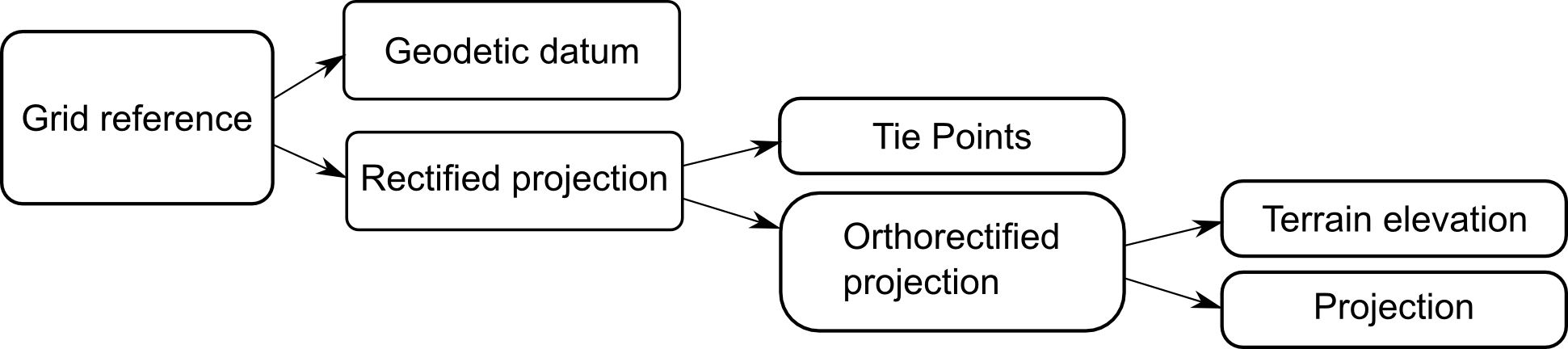
The data structure is illustrated in Figure 4, “The components of a rectified reference”.
Interfaces and classes used for rectification
Projections
As already mentioned, the central role is played by the ILcdRectifiedProjection. The interface offers access to two sets of points, called source points and target points. The source points are expressed
in the non-rectified world coordinates and the target points are expressed in the rectified world coordinates (see Figure 3, “Transformations from pixels to geodetic coordinates in a non-rectified grid”). The two sets of points are used internally to compute the parameters of the rectifying function. In addition, the interface
offers access to the internal projection.
There are a number implementations of this interface in LuciadLightspeed: TLcdRectifiedPolynomialProjection, TLcdRectifiedRationalProjection, and TLcdRectifiedProjectiveProjection. The polynomial projection applies a 2D polynomial of the form:
The rational projection applies a rational function of the form:
The projective projection applies a projective transformation of the form:
All classes take pairs of tie points as input, defined in (rectified/non-rectified) world coordinates. They internally compute the coefficients of the polynomials, minimizing the least-squares error of the mapping.
Raster referencers
The rectifying projections discussed in the previous section only work in world coordinates. For convenience, LuciadLightspeed
also provides a number of higher-level classes that allow you to create raster references starting from image points, defined
in pixel coordinates, and model points, defined in any georeference. The classes implement the interface ILcdRasterReferencer. The basic implementations only perform simple operations like rotations and translations. The more advanced implementations,
corresponding to the projections above, are TLcdPolynomialRasterReferencer, TLcdRationalRasterReferencer, and TLcdProjectiveRasterReferencer.
Program: Rectifying an image with the help of a raster referencer illustrates a typical usage scenario. Given image tie points expressed in pixel coordinates, and model tie points expressed in a given model reference, the raster referencer derives an appropriate model reference and bounds for the raster.
int imageWidth = 1000;
int imageHeight = 1000;

ILcdPoint[] imagePoints = new ILcdPoint[]{
    new TLcdXYPoint(0, 0),
    new TLcdXYPoint(1000, 0),
    new TLcdXYPoint(0, 1000),
    new TLcdXYPoint(1000, 1000),
    new TLcdXYPoint(126, 274),
    new TLcdXYPoint(983, 829)
};

ILcdModelReference modelPointsReference = new TLcdGeodeticReference();

ILcdPoint[] modelPoints = new ILcdPoint[]{
    new TLcdLonLatPoint(20.4, 30.8),
    new TLcdLonLatPoint(25.1, 30.6),
    new TLcdLonLatPoint(20.9, 35.7),
    new TLcdLonLatPoint(25.2, 35.3),
    new TLcdLonLatPoint(21.0, 31.9),
    new TLcdLonLatPoint(24.9, 35.0),
    };

int degree = 2;

ILcdRasterReferencer rasterReferencer =
    new TLcdPolynomialRasterReferencer(degree);

ILcdRasterReference rasterReference =
    rasterReferencer.createRasterReference(imageWidth,
                                           imageHeight,
                                           imagePoints,
                                           modelPointsReference,
                                           modelPoints,
                                           null);

ILcdModelReference modelReference = rasterReference.getModelReference();
ILcdBounds bounds = rasterReference.getBounds();
Once the raster reference and its bounds are known, the raster can be added to a model as shown in Program: Adding a raster to a model.
double pixelDensity = (imageWidth / bounds.getWidth()) *
                      (imageHeight / bounds.getHeight());
int defaultValue = 0;
ColorModel colorModel = ColorModel.getRGBdefault();

ILcdRaster raster = new TLcdRaster(bounds,
                                   tiles,//this is an ILcdTile[][]
                                   pixelDensity,
                                   defaultValue,
                                   colorModel);

ILcdModel model = new TLcd2DBoundsIndexedModel(modelReference,
                                               modelDescriptor);

model.addElement(raster, ILcdFireEventMode.NO_EVENT);
Limitations
Polynomial functions are notoriously unstable when their degree increases. For this reason it is recommended that you use only low-degree polynomials (2, maximum 3). Rational functions have the added problem of the denominator possibly becoming 0, which may make certain points unmappable.
Parametric rectification (orthorectification)
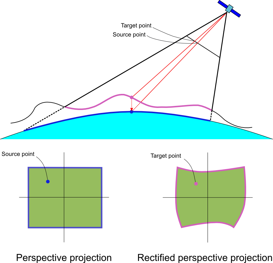
When both the imaging sensor parameters and a digital terrain elevation model are available, the distortion introduced by the terrain can be taken into account, as illustrated in Figure 5, “Image rectification when the sensor parameters and the terrain elevation are available”. If only the camera parameters would be available, a geodetic point located on the surface of the ellipsoid would be projected directly to a corresponding point in image coordinates (denoted as source point). However, due to the terrain elevation the geodetic point should actually mapped to a different position in the image: the target point. The process of canceling the distortions introduced by the camera projection and the terrain is sometimes called orthorectification.
Parameters related to the imaging sensor
The mapping from the 3D world to the camera’s 2D sensor can be expressed as a perspective projection. This projection is
implemented by the class TLcdPerspectiveProjection, which requires the following information:
-
the center of perspective
-
the principal point
-
the camera rotation around the principal axis
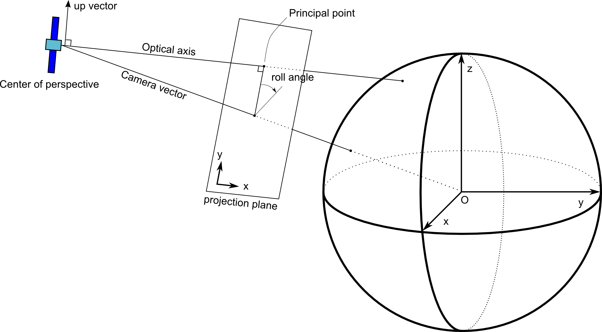
The center of perspective can be thought of as the sensor location, while the principal point is the foot of the perpendicular to the projection plane through the perspective center. Together, these two points define the principal axis (also known as optical axis) and the position of the projection plane. The principal point is also the origin of the projection plane.
The constructors of the TLcdPerspectiveProjection expect the center of perspective and the principal point to be expressed in geocentric coordinates. The camera rotation around
the principal axis can be expressed either as a roll angle or as an up vector. The roll angle is measured in degrees, clockwise
in the projection plane, relative to the plane determined by the camera vector and the optical axis - see Figure 6, “The parameters of the imaging sensor”. An up vector is a 3D vector orthogonal to the principal axis and parallel to the projection plane’s Y axis.
Including terrain information
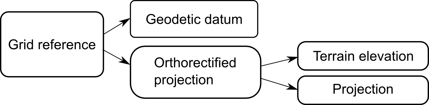
The distortion caused by the topographic relief is modeled in LuciadLightspeed as a projection called TLcdOrthorectifiedProjection. As with non-parametric rectification, this allows for a rectified reference to be used like any other grid reference. The
orthorectified projection combines the TLcdPerspectiveProjection presented in the previous section with elevation data coming from an ILcdHeightProvider - see Figure 7, “The components of an orthorectified and corrected grid reference”.
In its simplest form, the orthorectified projection behaves as a slightly modified version of the perspective projection itself (Program: Creating an orthorectifying projection from camera parameters and terrain elevation).
TLcdGeneralPerspective cameraProjection = new TLcdGeneralPerspective(
    0, 0, 10000,    // lon, lat, height
    20, -70, 0   // distance,azimuth, tilt
);
ILcdHeightProvider heightProvider =
    new TLcdFixedHeightProvider(1000, new TLcdLonLatBounds(-180, -90, 360, 180));
TLcdOrthorectifiedProjection orthorectified =
    new TLcdOrthorectifiedProjection(cameraProjection, heightProvider);
If you need to orthorectify an image that is already reprojected in a different coordinate system you can pass the existing
projection as the second argument of the TLcdOrthorectifiedProjection constructor:
ILcdProjection originalProjection = new TLcdEquidistantCylindrical();
TLcdOrthorectifiedProjection orthorectified =
    new TLcdOrthorectifiedProjection(cameraProjection,
                                     originalProjection,
                                     heightProvider);
Limitations
The current implementation of TLcdOrthorectifiedProjection cannot handle shadowed areas - low elevation terrain of which the visibility is obstructed by nearby high elevation terrain.
Shadowed areas result in local mapping discontinuities. Also, the projection cannot be successfully stored and restored from
a Properties object because the actual mapping is determined by the terrain elevation map. Attempting to store the projection properties
will save a single elevation sample, located at the principal point. When the projection is loaded back, that unique sample
is used for the entire projection.
Combining parametric and non-parametric rectification
Non-parametric rectification works well for large areas but cannot cope with localized distortions caused by the terrain.
On the other hand, the parametric rectification’s explicit modeling of the terrain produces very accurate results, but parametric
rectification is very sensitive to the quality of the camera parameters. For example, an error of a fraction of a degree in
the camera orientation can easily introduce errors of hundreds of meters at the ground level. Fortunately, the two methods
are complementary. By combining them, the overall results can significantly be improved. Any error in the camera parameters
can be corrected with just a few tie points, while the local terrain elevation is still taken into account. In terms of code
implementation it is sufficient to chain together the original projection, the TLcdOrthorectifiedProjection and the ILcdRectifiedProjection:
ILcdHeightProvider heightProvider =
    new TLcdFixedHeightProvider(1000, new TLcdLonLatBounds(-180, -90, 360, 180));
ILcdProjection original = new TLcdEquidistantCylindrical();
TLcdGeneralPerspective perspective = new TLcdGeneralPerspective(
    0, 0, 10000,    // lon, lat, height
    20, -70, 0   // distance,azimuth, tilt
);
ILcdPoint[] sourcePoints = new ILcdPoint[]{
    new TLcdXYPoint(0, 0),
    new TLcdXYPoint(1000, 0),
    new TLcdXYPoint(0, 1000),
    new TLcdXYPoint(1000, 1000),
    };

ILcdPoint[] targetPoints = new ILcdPoint[]{
    new TLcdXYPoint(-2.5, 0),
    new TLcdXYPoint(985, 1.2),
    new TLcdXYPoint(1.3, 1002),
    new TLcdXYPoint(988.3, 1002),
    };
TLcdXYBounds world_bounds = new TLcdXYBounds(-3, 0, 1000, 1002);

TLcdOrthorectifiedProjection orthorectified =
    new TLcdOrthorectifiedProjection(perspective,
                                     original,
                                     heightProvider);
TLcdRectifiedPolynomialProjection corrected =
    new TLcdRectifiedPolynomialProjection(2,
                                          sourcePoints,
                                          targetPoints,
                                          orthorectified,
                                          world_bounds);
TLcdGridReference gridReference = new TLcdGridReference(new TLcdGeodeticDatum(), corrected);
A visual illustration of the resulting coordinate transformations is presented in Figure 8, “The result of combining non-parametric and parametric rectification”.
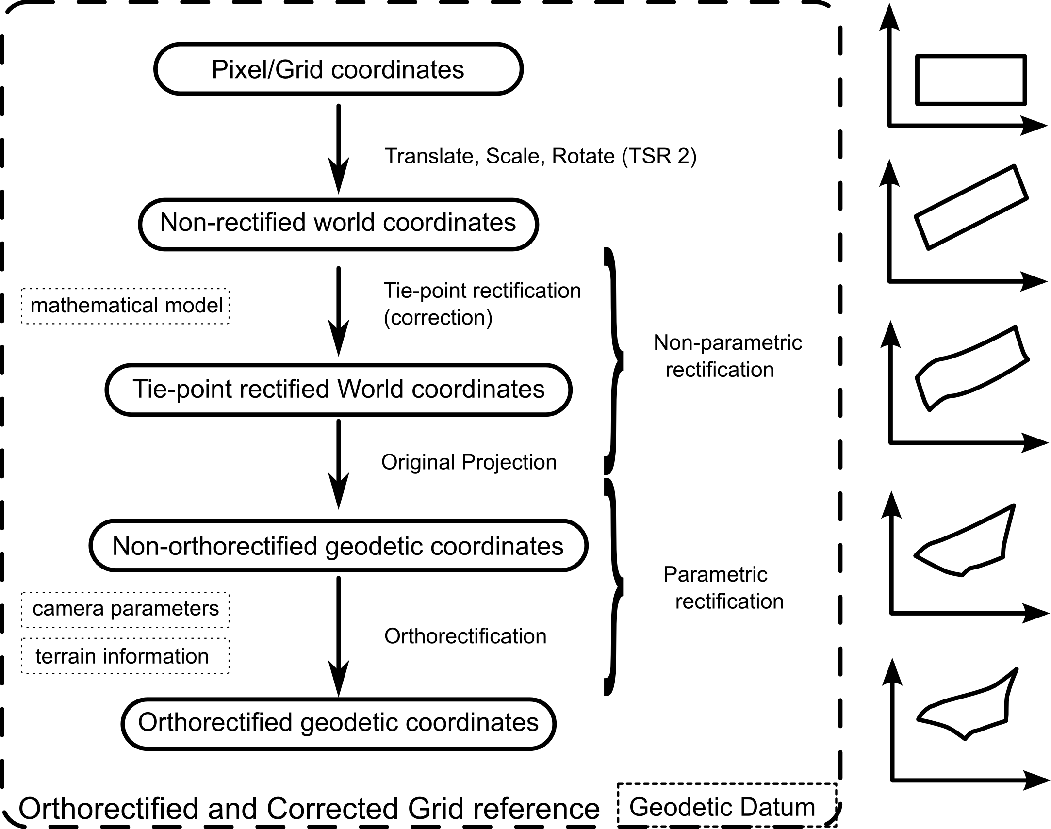
The final data structure is displayed in Figure 9, “The components of an orthorectified and corrected grid reference”.