LuciadFusion Samples
Browse samples per component: All installed
Highlighted samples
Lightspeed: Displaying dynamic data on a map and timeline
Lightspeed: Lidar visualization
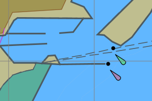
Lightspeed: Line Of Sight
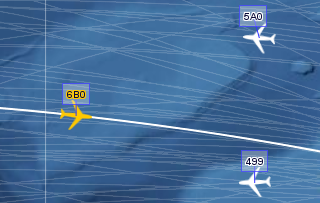
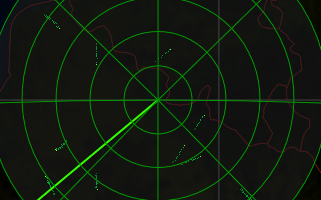
Lightspeed: Radar sweeps
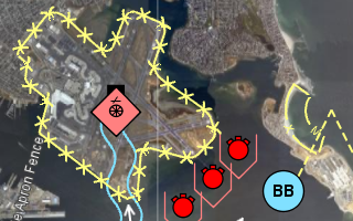
Lightspeed: display military symbology
Lightspeed: displaying S-101 data
Lightspeed: Decoding multiple format data
Lightspeed: Editing geometric shapes
LuciadFusion
Encoding GeoJson samples.encoder.geojson.Main
This is a command-line sample. Click More info for run instructions.
This command-line tool demonstrates how to decode vector data in various formats and export them as a GeoJson file.
Run the sample using the shell script in the samples folder:
encoder.geojson.bat <input_vector_data> <output_geojson>
The input consists of two parameters: (1) the path to the input vector file (for example, in SHP format), and (2), the path of the output GeoJson file.
Encoding MIF samples.encoder.mif.Main
This is a command-line sample. Click More info for run instructions.
This command-line tool demonstrates how to decode vector data in various formats and export them as a MIF file.
Run the sample using the shell script in the samples folder:
encoder.mif.bat <input_vector_data> <output_mif>
The input consists of two parameters: (1) the path to the input vector file (for example, in SHP format), and (2), the path of the output MIF file.
Encoding GeoTIFF samples.encoder.raster.geotiff.Main
This is a command-line sample. Click More info for run instructions.
This command-line tool demonstrates how to decode rasters in various format and encode them in GeoTIFF format, using a TLcdGeoTIFFModelEncoder.
Run the sample using the shell script in the samples folder:
encoder.raster.geotiff.bat [options] <input_raster> [...] <output_geotiff>
The input can be a single raster or a list of rasters that lie on a regular grid. The sample automatically figures out the structure of the grid and creates a composite raster that can be saved. The code may be generally useful for creating such composite rasters. They are more efficient to work with than the original unstructured list of rasters, for instance for analysis or for visualization.
The output GeoTIFFs are tiled and multi-leveled, and optionally compressed with JPEG compression. The default tile size is 256x256 pixels. The default number of levels is 5. The JPEG compression quality is a specified value between 0 and 1.
The supported options are:
-levels   <n>
-tilesize <n>
-jpeg     <f>
-bigtiff
GXY: Balloon samples.gxy.balloon.MainPanel
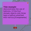
This sample demonstrates how to create your own balloons. Just click any of the domain objects to see an example of a balloon in action. Of the 4 domain objects 3 have a balloon attached to them.
Instructions
This sample demonstrates how to create your own balloons. Select a domain object to see an example of a balloon in action. Balloons are only shown when one domain object is selected.
One of the objects contains a balloon with a button that can be used to close itself. Another balloon shows an image, and another one shows a text label. The last domain object doesn't have a balloon attached to it.
You can move around balloons by dragging near their border. Balloons can be rescaled by dragging their lower right corner. The can also be closed by clicking the exit icon in the upper right corner.

Map raster values to colors samples.gxy.colormap.MainPanel
This sample shows you how to map raster data values to colors using TLcdColorMap, and how
to interactively customize such a map using TLcdColorMapCustomizer.
The sample shows elevation data that can be customized using the configuration panel.
Instructions
The color map customizer allows configuring the following:
- change the altitudes by clicking on them
- change the colors by clicking on the colored rectangles
- enable or disable gradient coloring
- enable or disable the linear scale
- in linear scale mode, drag the arrows around with the mouse
- add, remove, or re-initialize levels using the toolbar buttons
GXY: Asynchronous layer painting samples.gxy.concurrent.painting.MainPanel
This sample demonstrates the ability to paint asynchronously. It shows how to instantiate an asynchronously painted layer and a paint queue that handles the actual painting. The layer is then painted in the background, in a separate thread, so the painting no longer blocks the user interface.
It also illustrates how to automatically assign paint queues to the asynchronous layers by using several paint queue managers which can be activated one-by-one:
- The default paint queue manager, minimizing the number of paint queues.
- A paint queue manager based on the paint times of the layers. The layers will only share a paint queue if their average painting times are of the same magnitude.
- A paint queue manager using a fixed number of paint queue instances. The default number of paint queues is determined by the number of CPUs.
The sample shows a number of layers that are painted asynchronously. Layers sharing a paint queue have the same color in the layer control. For illustration purposes, some layers have a fixed paint time, which is indicated in between square brackets.
Instructions
Try panning and zooming with the mouse wheel. New layer contents are added after the operations. The layer control coloring shows which layers use the same paint queue. Switch the paint manager, and notice how the paint queue assignments change. The synchronous layers (in black) and the unmanaged layer stay the same.
The Translucent checkbox to the right on the map renders all content with a translucency of 0.5. This demonstrates how to modify the state of the wrapped layer.
GXY: Contours samples.gxy.contour.MainPanel
This sample demonstrates how to calculate and visualize terrain contours as polylines and complex polygons.
Instructions
Four different contour layers are available:
- labeled polyline contours
- polyline contours with the altitude in the line style
- polygon contours that contain each other
- disjoint polygon contours
GXY: Decoding multiple format data samples.gxy.decoder.MainPanel
This sample demonstrates the ability to load and visualize data from sources in
different formats by making use of ILcdModelDecoder and ILcdGXYLayerFactory.
A File and a URL action are configured to load data in almost every available format.
The sample uses a composite ILcdModelDecoder to decode the data into an ILcdModel.
After this, a composite ILcdGXYLayerFactory creates a layer that controls how
the ILcdModel of the loaded data is displayed.
The model decoders and layer factories are retrieved using a service look-up mechanism, and
contain both built-in and sample implementations.
The sample supports images that are not georeferenced if the images are described in a small *.rst
meta-file (see TLcdRasterModelDecoder).
The sample also includes a custom format (see the package samples.decoder.custom1) to show how to implement
your own model decoder.
A save action, only available when the sample is run standalone, allows you to save an
ILcdModel to its file if an ILcdModelEncoder is set to the ILcdModel.
Currently this is only done for the custom format.
Instructions
Open a file or URL by clicking the appropriate toolbar button or by dragging a file or URL onto the map. Load Washington DC spot satellite image ( .rst format ) and Washington DC streets ( .shp format ) and notice how the data overlap. Load mixed.txt, edit the shapes and save the model (only when run standalone).
GXY: Displaying element densities samples.gxy.density.MainPanel
This sample demonstrates how to display color-coded densities of data, by
means of a TLcdGXYDensityLayer.
The applet shows a set of flight trajectories above USA, with colors ranging from blue, for quiet regions, to bright white, for busy regions.
Instructions
Pan and zoom around. Notice that asynchronous painting ensures that the view stays responsive.
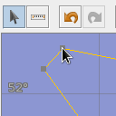
GXY: Editing geometric shapes samples.gxy.editing.MainPanel
This sample demonstrates how to interactively create and edit ILcdShape objects in an ILcdGXYView.
The toolbar contains buttons that create several shapes, by using different instances of
the TLcdGXYNewController2 controller.
Each controller has its own controller model, defining the type of
shape to create, in which ILcdGXYLayer to add it and how to add it.
The layers provide the necessary ILcdGXYPainter and ILcdGXYEditor instances to properly
render, create and edit any ILcdShape it contains.
Next to this, the panel at the right has the following configuration options:
- Rendering can be simplified by using straight lines (a pen setting)
- The shape outline/fill can be changed (a painter setting)
- New shapes can be defined in a geodetic (lon lat) reference, or a grid reference. Note that rhumb shapes cannot be defined in a grid reference.
- The sub-curve type of composite curves can be changed, even while creating the curve.
Instructions
- Click one of the new shape buttons in the toolbar and click on the map to create a new shape. For composite curves, you can start a new subcurve by selecting a shape in the drop down box.
- Edit a shape in one of the shape layers by dragging one of its points or segments. Notice how Geodetic shapes stay within their model reference (e.g. the earth) and wrap over the dateline, whereas Grid shapes are not bound by lon-lat coordinates.
- Using the CTRL (CMD on Mac OS) key, you can reshape objects. For example, for polylines and polygons, it allows you to add or remove points.
- Right-click on a point, polyline, or polygon and convert them into a buffer.
- Notice how very long geodetic and rhumb lines are not necessarily straight.
GXY: Editing with multiple modes samples.gxy.editmodes.MainPanel
This sample shows how to implement a multi-mode edit controller i.e. a controller that changes its state when you click on an already selected object. The controller is used in a painter/editor wrapper to change the painter/editor, allowing different editing behavior.
The controller supports 2 modes:
- DEFAULT: the default mode indicating the controller's standard behavior.
- ROTATION: the rotation mode of the controller.
To add the rotation behavior, a support class defines a number of abstract methods that need to be implemented for a specific shape:
- a method returning an object's current rotation
- a method returning the rotation center of an object
- a method that rotates an object
Instructions
The sample shows two polygons that can be rotated in their respective model references. To activate the rotation mode, select an object, and click once more on the object. Rotate the shape by grabbing and dragging one of the rotation handles. Click again on the object to cycle through the available modes. Click on a previously unselected object to reset the editing mode.
GXY: Geoid samples.gxy.geoid.MainPanel
This sample illustrates support in LuciadLightspeed for geoids. It shows an image containing the geoid heights of the EGM2008 datum (Earth Gravity Model, 2008). Blue colors indicate that the geoid heights are negative (geoid below the ellipsoid of the WGS84 datum). Green colors indicate that the geoid heights are positive (geoid above the ellipsoid).
The geoid heights are also displayed in a label on the toolbar.
Geoid heights are typically used behind the screens, in calculations with references that have geodetic datums based on geoids. They are relevant for elevation data, for instance, which are commonly defined with respect to a few standardized geoid models. For accurate computations, elevations above a geoid can then be transformed to elevations above an ellipsoid.
Instructions
Move the mouse and see how the geoid height changes.
GXY: Grids samples.gxy.grid.MainPanel
This sample demonstrates how to display grid layers in a GXY view.
The following grid layers are included:
- Lon Lat: a simple multi-level grid showing longitude and latitude lines. The lines are refined up to the second.
- Border: a maritime-style lon lat border grid. The coordinates are refined up to the degree.
- Georef: an alphanumeric multi-level grid based on longitude latitude lines. The lines are refined up to the degree. The labels denote 1-by-1 degree squares.
- XY: a grid based on an
ILcdXYWorldReference. The labels denote meters. - OSGR: sample implementation of a multi-level alphanumeric grid system. OSGR is only defined for the United Kingdom, and offers two levels.
Instructions
- Select a grid type and an appropriate projection
- Pan and zoom around. Notice how the grid and its labels adapt.
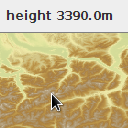
Height samples.gxy.height.MainPanel
This sample illustrates the use of height providers in LuciadLightspeed. It shows a raster containing height data. The height values of the data under the mouse cursor are displayed in a label on the toolbar.
The sample uses a view height provider to retrieve height values.
Instructions
Move the mouse over the raster and see how the height values change. Moving the mouse outside the raster will indicate that no height data could be found.
GXY: Highlighting domain objects samples.gxy.highlight.MainPanel
This sample demonstrates how to highlight domain objects. A custom controller looks at the domain objects under the mouse cursor and informs the relevant layer that an object should be highlighted.
Instructions
Hover above the cities and states. The city or state under the mouse will change color.
GXY: A painter/editor implementation samples.gxy.hippodromePainter.MainPanel
This sample contains an implementation of the ILcdGXYPainter and
ILcdGXYEditor interfaces for a new shape, a hippodrome,
which consists of two half circles connected by two lines. Instead of
using composition this sample demonstrates how to create a painter/editor
from scratch.
Note that this is sample code to demonstrate writing painters. If you need to model a hippodrome,
please refer to our ILcdGeoBuffer implementations.
The shape is defined by two points and a width. An XY and a lonlat shape is provided both of which can be handled by the painter/editor taking into account some precaution for the geodetic shape.
The painter supports painting in the following modes:
- painting the object in default and selected mode,
- painting the object while it is being edited,
- painting the object while it is being created.
- moving one of the defining points which results in a rotation, elongation of the shape,
- moving the whole shape,
- changing the width of the shape.
Instructions
This sample is mainly intended as a developer's guide to construct painters and editors from scratch. To create a new hippodrome, click on either of the two buttons in the toolbar. To edit a hippodrome,
- move one of the points by dragging the mouse starting from a point,
- move the whole shape by dragging the mouse starting from the outline,
- change the width of the shape by dragging the mouse starting from the outline with the CTRL (CMD on Mac OS) key down.
GXY: Basic icons samples.gxy.icons.MainPanel
This sample demonstrates LuciadLightspeed's abilities to display icons. These icons, painted by
a TLcdGXYIconPainter can be scaled using a world or pixel scaling mode. They can also
return an anchor point, which gives them an offset. The sample also demonstrates oriented
icons.
Instructions
You can dynamically change the scale and scale mode by using the controls in the 'Icon scaling options' panel. The pin icons represent cities. Notice how the tip of the pin is anchored to the city. Notice how every airplane has a different rotation: the rotation is automatically retrieved from the domain object.
GXY: Create Labeling Algorithm samples.gxy.labels.createalgorithm.MainPanel
This sample demonstrates the creation and usage of labeling algorithms and labeling algorithm
wrappers. MyLabelingAlgorithm is a labeling algorithm that tries to place all labels on the
domain object's anchor point.
There are three wrappers that can be combined with this algorithm and each other.
RotationAlgorithmWrapper: Rotates all labelsMorePositionsAlgorithmWrapper: Creates extra label placements to be tried by offsetting the label by a few pixels in each direction.LabelDetailAlgorithmWrapper: Adjusts the size of the font and amount of information to create more label placement possibilities.
Instructions
After starting the sample, it is possible to choose between two labeling algorithms:
The sample algorithm SampleLabelingAlgorithm and a default labeling algorithm. Use the
check boxes to enable/disable using more possible positions or changing the font size
during labeling. Also moving the slider adjusts the rotation of all labels.
GXY: Interactive labels samples.gxy.labels.interactive.MainPanel
This sample demonstrates how labels can be made interactive. The labels can be edited in the sense that they can be moved to a new location, as well as in the sense that they offer the user an interactive component that can be used to edit information related to the domain objects.
Instructions
Move the mouse over a label of a city. An interactive, editable label will be shown instead of the regular label. You can enter a comment for the labeled city in the text field. To apply the changes, press the Enter key or press the green tick mark at the top of the interactive label. To cancel the outstanding changes, press the red 'cancel' icon at the top of the label or press the Escape key.
The interactive label can be moved by clicking and dragging on the title bar of the interactive label.
GXY: Offset icons samples.gxy.labels.offset.MainPanel
This sample demonstrates LuciadLightspeed's abilities to display icons at a certain offset. These
icons, painted by a regular ILcdGXYPainter, are offset with respect to the domain object.
This offset can be dynamically changed using the mouse.
It also shows how the used labeling algorithm can be configured to drop labels together.
Instructions
You can dynamically change the offset of the icon by selecting a city, and then dragging the icon while keeping the 'Control' button pressed.
GXY: Basic Labeling samples.gxy.labels.placement.MainPanel
This sample demonstrates the asynchronous label placer and the default labeling algorithms.
Labeling algorithms take into account the
labels that are already placed to avoid overlap.
An ILcdGXYLayer will therefore most likely have less labels painted
when it is at the bottom than when it is at the top of the ILcdGXYView.
Instructions
To see the effects of the labeling algorithms select a layer, by clicking it in the layer control and:
- change the layer's visibility
- set the layer labeled/not labeled
- move the layer up/down
GXY: Street Labeling samples.gxy.labels.streets.MainPanel
This sample demonstrates LuciadLightspeed's abilities to paint and label streets. Highways are labeled using an icon, while city streets (zoom in on Washington DC) are labeled using text labels.
Instructions
Zoom in and out to see multiple levels of detail on the map. The USA region contains highway data, and the Washington DC region contains streets data.
Magnetic north samples.gxy.magneticnorth.MainPanel
This sample shows you LuciadLightspeed's capabilities regarding the magnetic north.
The magnetic north does not coincide with the true north. The difference between the magnetic and true north is called magnetic declination and depends on your position in space and time. There are different mathematical models to calculate and predict the magnetic north, each with their own lifespan. LuciadLightspeed comes with the two most popular models: WMM and IGRF.
The sample shows a compass control for the magnetic north, and iso lines of constant magnetic north declination.
Instructions
Click on any place on the map to center on that point and rotate the map so that the top points towards the magnetic north. Notice that the magnetic north compass will point straight up. Right-click to reset the custom rotation again. Zoom in on a magnetic declination line. The readout at the bottom of the map shows the exact declination value for the mouse location. The magnetic value at the center of the map should be the difference between both compasses.
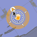
GXY: On Map Navigation Controls samples.gxy.navigationcontrols.MainPanel
This sample demonstrates how to create, customize, add on map navigation controls over a 2D view.
Instructions
The default controls are in the top right corner when you run the sample. Drag the outer ring of the upper part to rotate the view (you can hold down the CTRL (CMD on Mac OS) button to constrain rotation to multiples of 15 degrees). Click on the North symbol of the outer ring to return the view to the original rotation. Press and hold anywhere in the circle with the hand symbol to pan the view. The lower part allows you to zoom in and out.
On the left you can find a customized configuration. In the alternative configuration, the controls are split and the two sub-components are added in different places. Furthermore, the zoom component is now always emphasized, not only when the mouse is over it and the compass component can be relocated by dragging it with the right mouse button pressed.
GXY: Offscreen view samples.gxy.offscreen.Main
This is a command-line sample. Click More info for run instructions.
This command-line tool demonstrates how to create an off-screen view, display some decoded data in it, and save the result as a GeoTIFF file.
Run the sample using the shell script in the samples folder:
gxy.offscreen.bat <input_file> <output_geotiff>
The input data can be in a variety of formats: SHP, MIF, MAP, GeoTIFF, etc. The output GeoTIFFs are 1024x1024 pixels, tiled (256x256 pixels) and multi-leveled (3 levels), and compressed with a lossless compression scheme. All of these settings can be changed in the sample code.
GXY: Overview map samples.gxy.overview.MainPanel
This sample demonstrates the use of a TLcdGXYOverviewController and the
sharing of layers between multiple ILcdGXYView objects.
It consists of one main ILcdGXYView (TLcdMapJPanel) in the center and an overview map
(TLcdMapJPanel) in the top right. The overview map remains focused on the USA and
also displays a Rectangle that corresponds as much as possible to the area visible
in the main view. Dragging the Rectangle in the overview or creating a new one makes
the main view display data that are in the Rectangle. This Rectangle is updated
each time the visible area in the main view changes (e.g. when panning or zooming).
The overview displays the same ILcdModels using the same ILcdGXYLayers used in the main view.
Since an ILcdGXYView automatically listens to any property change of its
ILcdGXYLayer objects, any change of those properties via the layer control
will show in both views.
Instructions
Drag the Rectangle in the overview or create a new one. Pan and zoom in the main view: the Rectangle overview will update itself automatically. Remove a layer and notice that it is removed from both views.
GXY: Painter styles samples.gxy.painterstyles.MainPanel
This sample shows how to paint polylines and polygons with rounded corners and how to change the stroke and fill style.
The functionality to paint a polyline or polygon with rounded corners is provided by
TLcdGXYRoundedPointListPainter.
To fill shapes with a solid color, TLcdGXYPainterColorStyle is used.
To fill shapes with a hatched pattern, TLcdGXYHatchedFillStyle is used.
To render outlines with a simple, dashed stroke, TLcdStrokeLineStyle is used.
To render the shapes with a pattern-based stroke, TLcdGXYComplexStroke is used.
This java.awt.Stroke implementation allows to use an AWT Shape array as pattern to
render a shape.
The sample also illustrates halo effects.
A halo is an outline of constant width and color around shapes or text, which is typically drawn in
a contrasting color to ensure that the shapes or text are clearly visible on any background.
For shapes, the halo effect is obtained by wrapping an ILcdGXYPainter (in this case,
the TLcdGXYRoundedPointListPainter) into a TLcdGXYHaloPainter.
Instructions
- Select a polyline or polygon to show style properties. The select controller's sensitivity has been increased to improve the selection of lines with thick linestyles.
- Change the roundness through the slider.
- Choose a different pattern for the complex stroke, adjust the repeating factor, or adjust the gap between the pattern shapes
- Change the tolerance. The tolerance defines how large the cut-off error may be when placing the patterns; its effect is most visible in sharp corners. If the error is too high, a fallback stroke is used.
- Change the 'Allow split' option. When no split is allowed, the stroke should only contain contiguous full pattern sequences (thus, pattern 1 times its repetition factor followed by pattern 2 times its repetition factor). When there is not enough space for a full sequence, a fallback stroke is used.
- Change the halo color, and increase/decrease the halo width.
- Add one or more points to an existing polyline by CTRL-clicking on the line
- Create a new polyline using the button in the toolbar. The polyline will take over the current style.

GXY: Printing samples.gxy.printing.MainPanel
This sample demonstrates how to print a component containing a view,
using the TLcdGXYViewComponentPrintable.
Instructions
The sample creates a page layout containing the view and some decorations. You can preview the page or print it directly using the buttons in the toolbar.
GXY: Rectifying rasters samples.gxy.rectification.MainPanel
This sample demonstrates the ability to combine parametric rectification - using camera and terrain information - and non-parametric rectification - using user-defined tie-points.
Instructions
The left panel displays a non-modified version of the image currently being processed, together with a set of tie points. The right panel displays several layers, from bottom to top:
- the world background data
- the digital elevation map (terrain)
- the input raster in its unmodified geographical reference (original raster)
- the result of parametric rectification (orthorectified raster)
- the result of non-parametric rectification (tie-point corrected raster)
- the tie points
- a layer containing data that can be used to verify the accuracy of the rectification
The default data is a simulated satellite photo of the city of Ithaca, NY. Due to the slanted viewing direction, the position of the original picture is distorted by a variable amount compared to the real position. The size of the distortion depends on the local terrain elevation - this can be verified by comparing the position of roads in the original raster with their actual position displayed by layer "109rds".
By taking into account the viewing direction and the variable terrain elevation, the sample creates an initial orthorectified version of the raster, which corrects most of the positioning errors. The user may further correct a copy of this raster by fine-tuning a set of tie points.
An initial set of tie points are shown in the left and in the right panels. Selecting a point in one panel will display the corresponding tie point in the other panel. Tie points in both panels can be dragged to other locations. This will trigger a remapping of the corrected image in the right panel, so that the tie points appear in approximately the same location relative to the raster.
New tie points can be added in the left panel by selecting the "Create new tie point" controller. Every time a new point is added in the left panel, a corresponding tie point is added to the right panel, at approximately the same raster coordinates (a small difference may be observed for highly warped rasters).
Existing tie points can be deleted by right-clicking on them and choosing "Delete" from the context menu. If fewer than 3 points are available, the raster is no longer updated.
By default, the mapping is done using a polynomial function. You may choose a rational function or a projective function instead, by selecting the "Edit raster projection parameters" action. You can also choose the maximum degree of the polynomial(s) used by the selected function. Note that polynomials of higher degree (3 or 4) are highly unstable and may produce strange warping effects. The number of required tie point pairs varies with the degree of the polynomial(s). If an insufficient number of tie points is defined, the function will automatically decrease the degree(s) used.
When you are satisfied with the rectification you may save a re-sampled version of the raster using the reference of the right-panel view using the "Save the raster in view's reference" button.
The sample can open existing single-level referenced GeoTIFF files, or non-referenced images (tif, png, gif, bmp, jpg). If the image is not georeferenced, it is placed at a default location, together with four initial tie points in the corners.
The open and save options are not available when the sample is running in a browser.
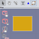
GXY: Displaying shapes samples.gxy.shapes.MainPanel
This sample shows how to programmatically create and display a model.
It reveals how to create an ILcdModel, how to populate it with ILcdShape objects,
and how to display that data in an ILcdGXYLayer on the ILcdGXYView.
Instructions
The sample shows a polyline, a polygon, and a point visualized by an icon. Try selecting and editing the shapes.
GXY: Painter, shape composition samples.gxy.shortestDistancePainter.MainPanel
This sample demonstrates how to create a composite ILcd2DEditableShape and a
suitable ILcdGXYPainter and ILcdGXYEditor for that ILcd2DEditableShape.
The class ShortestDistanceShape is a composition of a TLcdLonLatPolyline and
a TLcdLonLatPoint around this polyline. The class ShortestDistanceShape knows
how to calculate the ILcdPoint on the geodesic TLcdLonLatPolyline that is the
closest to the TLcdLonLatPoint.
The class ShortestDistancePainter implements ILcdGXYPainter and ILcdGXYEditor
and is used for painting and editing ShortestDistanceShape objects.
Existing painters for the composed shape object are used for painting,
TLcdGXYIconPainter for the TLcdLonLatPoint and TLcdGXYPointListPainter for
the TLcdLonLatPolyline. For painting the shortest distance path of the
TLcdLonLatPoint to the TLcdLonLatPolyline the utility ILcdGXYPen is used.
Instructions
The painter-editor allows to move the TLcdLonLatPoint or a point of the
TLcdLonLatPolyline of the ShortestDistanceShape object to any location while
constantly showing the shortest distance path of the TLcdLonLatPoint to
the TLcdLonLatPolyline.
GXY: Visualizing statistical information samples.gxy.statisticalPainter.MainPanel
This sample shows how to visualize shapes based on their domain object properties. A custom painter provider displays counties as polygons that are colored according to population density. Icon-based labels show different size rectangles depending on the population change.
Instructions
You can verify the visualization by double-clicking on a shape to examine its properties.
Model in a table samples.gxy.swingTable.MainPanel
This is a sample for displaying an ILcdModel's elements in a JTable.
All the domain objects implement ILcdDataObject, which means they have a data type with
a set of properties associated to each of them.
We load several ILcdModel which are displayed/represented in both
the TLcdMapJPanel and the JTabbedPane (i.e. each ILcdModel is represented
in 2 different views). For each ILcdModel, there is a
corresponding ILcdGXYLayer in the map and a JTable in the JTabbedPane.
The column names of each JTable correspond to the attributes names,
the rows correspond to the attribute values.
A mediator is used to synchronize the map and table selections.
Instructions
- Select one or more rows in one of the tables. Notice how the domain objects are made visible and selected in the map.
- Select one or more objects on the map. Notice how the corresponding table rows are selected as well.
GXY: Tooltips on the map samples.gxy.tooltip.MainPanel
This sample contains a custom implementation of ILcdGXYController, which
displays tooltips for objects under the cursor. The text of the tooltips is
obtained via the ILcdDataObject interface. The applyOnInteract2DBounds()
method of ILcd2DBoundsIndexedModel is used to locate the object under the
mouse cursor.
Instructions
Hover over a city or state and a tooltip will pop up after a short while.
GXY: Touch controller samples.gxy.touch.basic.MainPanel
This sample demonstrates the touch-based navigation, selection and ruler controllers in a GXY view. The controllers are shown in the toolbar at the top. The leftmost controller is a context sensitive selection and navigation controller.
The second controller only deals with navigation. It features one finger panning, and two finger panning, zooming and rotating (at the same time).
The third is a ruler controller. It works similar to the mouse based ruler controller, creating a polyline on the map that will display the length of each segment as well as the total length.
This sample features large buttons to allow easy manipulation with fingers instead of a mouse as input device.
Instructions
Using the select controller, you can touch objects to select them, pan around by dragging the map, or zoom and pan by dragging two fingers. A number of modifier buttons are available to change the selection behavior:
- The first button enables multi-object selection by dragging a rectangle around objects. By default, dragging pans the map.
- The second button toggles what happens when you touch selectable objects: select them (and deselect all other objects), add them to the selection, or remove them from the selection.
- The third button enables showing a pop-up with the objects under your finger. The pop-up allows you to choose the object to select.
For the pan controller, drag one finger to pan, and two fingers to simultaneously pan, zoom and rotate the map.
To add points to the ruler controller's measurement, touch and lift your finger. Here as well a number of buttons are added to the map:
- The blue arrows undo/redo a step.
- The green V commits the created polyline. This switches the ruler controller to edit mode.
- The red cross clears the polyline and allows you to start again.
GXY: Create and edit shapes with a touch device samples.gxy.touch.editing.MainPanel
This sample demonstrates how to create new ILcdShape objects and edit
existing ILcdShape objects in an ILcdGXYView using a touch device.
The functionality available here is very similar to the functionality demonstrated by the editing sample. The main difference is that the controllers now interpret touch input instead of mouse input. This allows you for instance to translate an object using the edit controller with one finger and pan the view with another finger at the same time. The same goes for the controllers creating objects. Another issue is the lack of modifier buttons (on keyboard and mouse). To compensate the touch controllers have been extended with some on-map buttons. The edit controller has:
- the same buttons as the select controller (see the touch.basic sample)
- a button that toggles between translate and reshape behaviour when editing.
- two buttons (blue arrows) to perform an undo respectively a redo operation. An undo will remove a previously placed point, while a redo will place a removed point again.
- a (green) button to commit a shape under construction. This is only relevant for polylines and polygons. Other shapes will be committed when the necessary amount of points is placed.
- a (red cross) button to cancel the current shape under construction, removing all points.
Instructions
- Touch or click on one of the new shape buttons in the toolbar and touch the map to create a new shape. The point will only be placed when you release the touch. When you have placed of number of points (how many depends on the shape), an object will be added to the drawing layer, and the edit controller will be activated. For composite curves, you can start a new subcurve by selecting a shape in the drop down box.
- Edit a shape in the user layer by dragging one of its points or segments
GXY: Generating touch events samples.gxy.touch.touchEvents.MainPanel
This sample demonstrates how TLcdTouchEvents can be created from hardware events. The sample
simulates touch hardware generating hardware events. These events are intercepted and
converted into touch events that can be used by LuciadLightspeed. After that they are dispatched.
Instructions
After opening the sample, touch events will be generated automatically. They pan, zoom and rotate the view.
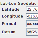
Grid systems samples.gxy.transformation.geodeticToGrid.MainPanel
This sample demonstrates the ability to display a geodetic location which can
be expressed based on different ILcdGeodeticDatum and express its coordinates
in some commonly used grid reference systems and some lon lat formats.
Instructions
Move the displayed icon and see how its coordinates change.
There are two text fields which contain the geodetic latitude and longitude respectively. The latitude and the longitude are represented in a certain format which can be changed. Values have to be entered in this format too. The geodetic coordinate is with respect to a certain geodetic datum which can be altered. In the grid coordinates panel are the (x,y) grid coordinates of this geodetic LatLon coordinate according to some commonly used grid coordinate systems.
Changing the geodetic datum or the UTM zone will affect only the geodetic coordinate or the UTM coordinate. Since the geodetic datum of the projection in the map component is kept the same as the geodetic datum of the grid calculator, the icon will move slightly too.
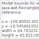
GXY: Model-world and world-view transformations samples.gxy.transformation.mouseToGeodetic.MainPanel
This sample contains a custom implementation of ILcdGXYController, which
transforms a rectangle dragged by the user (in view coordinates) into
model coordinates. The mouse location is also
converted into an arbitrary model reference (a grid reference with a
polar projection for the north pole).
Instructions
Drag a rectangle on the map, and see the coordinates of its counter part in model coordinates, below the map. The last mouse drag or mouse click location is also expressed in another model reference.
GXY: Undo capabilities of LuciadLightspeed samples.gxy.undo.MainPanel
This sample demonstrates the undo support of LuciadLightspeed. It is based on the "shapes" sample and makes it possible to undo changes made to the domain objects.
Instructions
To witness the undo support, perform the following steps:
- Activate the edit controller using the leftmost button in the toolbar.
- Make some changes by dragging the polyline or one of its handles.
- Create one or more new polylines using the new polyline controller in the toolbar.
- Click the undo button in the toolbar and the changes you made will be reverted.
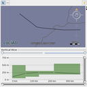
GXY: Vertical view samples.gxy.vertical.MainPanel
This sample demonstrates the use of the vertical view package. The 2D view in the upper part contains two layers: a background layer with a map of the world countries and a layer that contains two flights. Each flight is modeled as a list of 3D points. The 2D view only uses the first two coordinates(X,Y) of each of the points.
The vertical view in the lower part is used to display the vertical profile of
the flight that is selected in the 2D view. Apart from this profile,
a number of sub-profiles associated to it can be shown in a vertical view.
In this case, only one sub-profile is associated to the view: the air route.
FlightVVModel, an implementation of ILcdVVModel holds the main-profile points
and the information about the sub-profile.
Instructions
Select a flight. A vertical marker is shown in both views. Change the height of the flight by dragging its points up or down. You can zoom the X and Y axes by using the sliders to the right and at the bottom. You can disregard flight points at the left or right of the flight using the sliders at the top. Finally, the panel at the right allows you to select the altitude unit.
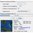
Preprocessing 3D terrain samples.earth.preprocessor.MainPanel
This sample demonstrates the use of TLcdEarthTileRepositoryPreprocessor. This sample
provides a simple user interface for creating, loading and saving 3D terrain
metadata and preprocessing it to an Earth tile repository.
Instructions
To preprocess data as a 3D terrain to an Earth tile repository you need to:
- Define the terrain metadata
- Configure the preprocessor
The terrain metadata consists of a number of assets (that is source data files) and a geographic reference. Add some assets to the metadata by using the button at the bottom of the panel. You can either select individual files that need to be preprocessed or a directory that contains the files that need to be preprocessed. Once the assets are loaded they will appear in the metadata panel and their bounding box will appear on the map. For image assets you can also optionally set a clipping shape to limit the preprocessed part. This can for example be used avoid preprocessing a border that is present in the asset. You can save the terrain metadata (for example for using with the Earth On-the-fly sample) using the button below the map. Finally you can change the geographic reference of the terrain using the combo box at the top of the metadata panel. Typically this geographic reference is the one that will most often be used when visualizing the terrain repository.
The repository where the assets should be preprocessed to must be configured before the preprocessor can be started. You can optionally also change the data type that must be preprocessed and enable texture transparency. After pressing the start button the preprocessing progress can be tracked in the progress panel and on the map. The preprocessor can be stopped at any time and resumed again using the buttons in the progress panel.
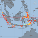
Filtering data using the OGC Filter API samples.ogc.filter.model.MainPanel
This applet demonstrates the ability to filter data using the OGC Filter API. A layer showing earthquakes is added to the view on which a filter is configured. The layer filter is created from an OGC filter, which is created from a combination of three OGC conditions: 'a less than' for the magnitude, a temporal for the time period and a bounding box condition of a country.
The OGC conditions are expressed programmatically using the OGC Filter API. The creation of the OGC conditions is done in EarthQuakeFilterModel#createCombinedCondition. If there is a change in one of the parameters for the OGC conditions, a new OGC filter is created and converted to an ILcdFiltered by means of a filter evaluator. This conversion code can be found in MainPanel#addData.
Instructions
Use the controls in the filter configuration panel to adjust the different parameters of the filter.
Filtering data using the OGC Filter XML Decoding facilities samples.ogc.filter.xml.MainPanel
This applet demonstrates the ability to filter GML data using the OGC Filter XML decoding and evaluation facilities.
It displays all the countries of the world and the same data, with a filter applied in another layer.
Instructions
Enter a filter manually in the text area at the bottom or click the load button to load a predefined filter from the list.
Click the apply button to apply the filter to the countries layer. The filtered layer will display all countries that pass the filter.
Double-click on a country in order to view its related features and compare them to the filter.
Command-line sample Tiling Engine samples.fusion.engine.Fuser
This is a command-line sample. Click More info for run instructions.
This command-line sample demonstrates how to fuse a single coverage from one or more input data sources. It illustrates both basic and advanced usage of the fusion engine. It has extension points that allow subclasses to customize it further. It can be used as a stand-alone command-line fusion tool in scripts. Because of 32-bit VM restrictions, it uses a default maximum heap of 768 MB (-Xmx768m), which may be too limited to fuse large data sets such as the NOAA ENCs. For a 64-bit VM, you may want set this to higher value in the sample's startup script, for example -Xmx1500m.
Run the sample using the shell script in the samples folder:
fusion.engine.bat -s:<source> -t:<target-tile-store>
Instructions
For a detailed list of command-line options, run the sample without arguments.
The minimal arguments are the input data source(s) and the target Tile Store URI:
"-s:<source>"The input data source(s), which may be a single file or a directory."-t:<target-tile-store>"The target Tile Store, which may be a local directory ("file:" URI) or a remote Tile Store ("http:" URI).
For example, "fusion.engine.sh -s:/my/input/data/sources -t:http://my.server:8081/LuciadFusion/lts"
will create a coverage using all the input data found in /my/input/data/sources.
The coverage and assets will have a generated UUID as ID, and no name.
Typically, you want to specify some options for assets and coverage. Options for assets start with
"-a:", options for the coverage start with "-c:".
For example,
"fusion.engine.sh -s[0]:/my/input/data/background.tif" -s[1]:/my/input/data/california.jp2
                              -a[0]:id:background.tif -a[1]:id:california.jp2 -c:id:california
will create a coverage "california" from two input data sources. The indexes determine the order: "california.jp2"
will be on top of "background.tif".
When you use this sample in a script, for example to regularly re-fuse a specific coverage, you may want to consider
the "-overwrite" option.
Without it, fusion would resume from checkpoint if a previous fusion was unfinished, or do nothing if a previous
fusion was finished.
Command-line sample Tiling Engine with custom ArcInfo ASCII Grid format samples.fusion.engine.format.Fuser
This is a command-line sample. Click More info for run instructions.
This command-line sample demonstrates how to plug in a custom raster format into the fusion engine.
It illustrates how support for ArcInfo ASCII Grid can be added by extending the
fusion.engine sample.
Run the sample using the shell script in the samples folder:
fusion.engine.format.bat -s:<source> -t:<target-tile-store>
Instructions
For a detailed list of command-line options, run the sample without arguments.
See also the fusion.engine sample for detailed instructions.
The minimal arguments are the input data source(s) and the target Tile Store URI:
"-s:<source>"The input data source(s), which may be a single file or a directory."-t:<target-tile-store>"The target Tile Store, which may be a local directory ("file:" URI) or a remote Tile Store ("http:" URI).
For example, "fusion.engine.sh -s:/my/input/data/sources.asc -t:http://my.server:8081/LuciadFusion/lts"
will create a coverage using all the input data found in /my/input/data/sources.
The coverage and assets will have a generated UUID as ID, and no name.
Command-line sample Point Cloud Pre-processor samples.fusion.pointcloud.PointCloudPreprocessorTool
This is a command-line sample. Click More info for run instructions.
This command-line sample demonstrates how to pre-process one or more input files into a single point cloud. It illustrates both basic usage of the pre-processor. It can be used as a stand-alone command-line tool in scripts. Because of 32-bit VM restrictions, it uses a default maximum heap of 768 MB (-Xmx768m), which may be too limited to process large data sets. For a 64-bit VM, you may want set this to higher value in the sample's startup script, for example -Xmx2g.
Run the sample using the shell script in the samples folder:
fusion.pointcloud.bat --input=<source> --output=<target-directory>
Instructions
For a detailed list of command-line options, run the sample without arguments.
The minimal arguments are the input data source(s) and the target path:
"--input=<source>"The input source, which may be a single file or a directory."--output=<target>"The target directory, which will be created if necessary.
For example, "fusion.pointcloud.sh --input=/my/input/data/sources --target=/my/output/pointcloud"
will create a point cloud store using all the input data found in /my/input/data/sources.
The output of this process can be imported into LuciadFusion Studio by adding the entire output directory as a "Data Root". Once the data root is crawled, you should be able to see a new data entry that represents the preprocesed dataset in your "Data" tab. To serve it, create a new Service using this dataset, and set the service type to "OGC 3D Tiles".
The preprocessed output can also be opened directly in a Lightspeed-based client such as Lucy. To do this, open the "tileset.json" found in the root of the output directory.
When you use this sample in a script, for example to regularly re-fuse a specific coverage, you may want to consider removing the target directory first. Without this, the preprocessor would add data from the input sources to the existing point cloud, or do nothing if all of the input sources were already to the point cloud previously.
Exporting data to GML31 samples.encoder.gml3.Main
This is a command-line sample. Click More info for run instructions.
This sample illustrates how to data in SHP, MIF or MAP formats can be transformed and exported as GML31 data.
Run the sample using the shell script in the samples folder:
encoder.gml3.bat [-gmlschema gmlSchema] [-xmlschema xmlSchema] [-namespace namespace] vectorFile resultFile
These are the parameters to pass:
- gmlSchema: the location of the GML schema to be encoded in the xsi:schemaLocations attribute
- xmlSchema: the location of the XML-SCHEMA schema to be encoded in the xsi:schemaLocations attribute
- namespace: the target namespace, if none is available.
- vectorFile: the name of a vector file that is to be converted
- resultFile: the name of the output file
Transforming data to and from GML samples.transformation.gml.GMLTransformationDemo
This is a command-line sample. Click More info for run instructions.
This sample uses the FlightPlan data model from the LuciadLightspeed fundamentals as source model. It shows how this data model can be transformed into a GML data model. It shows how the GML application schema can be generated. It then encodes a model containing flight plans as a GML document. Then this document is decoded back into a model containing flight plans.
Run the sample using the shell script in the samples folder:
transformation.gml.bat
Encoding JPEG2000 samples.encoder.raster.jpeg2000.Main
This is a command-line sample. Click More info for run instructions.
This command-line tool demonstrates how to decode rasters in various formats and encode them in JPEG2000 format, using a TLcdJPEG2000ModelEncoder.
Run the sample using the shell script in the samples folder:
encoder.raster.jpeg2000.bat [options] <input_raster> <output_jpeg2000>
The supported options are:
-levels   <n>
-layers   <n>
-quality  <f>
-lossless
-tilesize <width> <height>
GXY: displaying KML data samples.decoder.kml22.gxy.MainPanel
This sample demonstrates how to load and display KML data on a map.
Instructions
The sample will automatically load a basic KML file containing most KML features, and fit the map on the data.
The model content tree next to the map is a tree-based structure showing the contents of all KML files that are currently displayed on the map.
Objects can be selected either via the map or via the model content tree. When an object is selected a balloon will pop-up, displaying additional information on the object.
The sample will automatically resolve network links in KML files, and refresh the model contents if a refresh mode is specified in the link.
When KML files containing time information (timestamp, timespan) are loaded, a time toolbar will become visible, showing the time interval for which data is available. The time slider can be used to control which data should be shown on the map.
Lightspeed: displaying KML data samples.decoder.kml22.lightspeed.MainPanel
This sample demonstrates how to load and display KML data on a map.
Instructions
The sample will automatically load two KML files:
- a file containing Collada data, representing the town hall of Leuven.
- a basic KML file containing most KML features.
The model content tree next to the map is a tree-based structure showing the contents of all KML files that are currently displayed on the map.
Objects can be selected either via the map or via the model content tree. When an object is selected a balloon will pop-up, displaying additional information on the object.
The sample will automatically resolve network links in KML files, and refresh the model contents if a refresh mode is specified in the link.
When KML files containing time information (timestamp, timespan) are loaded, a time toolbar will become visible, showing the time interval for which data is available. The time slider can be used to control which data should be shown on the map.
Convert models into KML models and save them into KML files samples.encoder.kml22.KMLConverter
This is a command-line sample. Click More info for run instructions.
This sample demonstrates how to convert models into KML. The KML format is particularly useful for sharing a situational map with a broader set of stakeholders, who do not necessarily have access to LuciadLightspeed, but can open KML data in other map visualization tools. LuciadLightspeed allows you to convert map data into KML. This sample illustrates one way to convert vector data into KML and customize the conversion. It gives you full control of the style and the geometry information that will be converted in the KML model. The model encoder TLcdKML22ModelEncoder can then export the KML model.
Run the sample using the shell script in the samples folder:
encoder.kml22.bat
Run the sample to convert the files and the in-memory model into KML. The three new KML files are located in the Kml directory inside the data resources folder for the samples. You can visualize the KML files in the general decoder samples, the KML decoder samples, or any KML visualization tool.
First, the KML encoding sample decodes a SHP file representing tracks, and converts a subset of the tracks into a KML model. The KML model is then encoded in a file. Another SHP file representing the USA states is also decoded, and some states are encoded in KML. Next, the sample creates an in-memory model of airspaces. Each airspace is an extruded shape with a circle or a polygon as its base shape. The airspace model is also converted into KML and encoded.
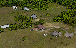
Lightspeed: Lidar visualization samples.lightspeed.lidar.MainPanel
This sample illustrates how Lidar data from .las files can be visualized in a Lightspeed view.
With this sample, you can open one or more .las files and apply different styling.
The following styling options are available if at least one layer supports it:
- Color: uses the color information available in the file.
- Height: shows a color gradient over the combined height range of all layers.
- Classification: shows a different color per class.
- Intensity: shows greyscale gradient based on the intensity available in the file.
- Infrared: shows a color gradient based on the infrared information available in the file.
Additionally, a shading technique to enhance depth perception is enabled by default. Using the controls in the panel, the settings can be changed:
- Enhance: the checkbox enables or disables the shading technique
- The thickness slider alters the thickness of the applied shade
- The strength slider alters the strength of the applied shade
- The color chooser changes the color of the applied shade
Instructions
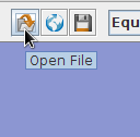
Open .las files using the "Open File" icon, or by dragging files onto the sample.
Change the styling and filtering using the panel on the right. The styling will be applied to the layers that support it. Layers that don't support it use Height styling.
Change the depth perception settings using the panel on the right. The settings will be applied to all layers.
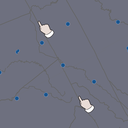
GXY: Clustering samples.gxy.clustering.MainPanel
This sample demonstrates how to introduce clustering in a GXY application
using
TLcdTransformingModelFactory and
TLcdClusteringTransformer.
The sample contains a large number of recorded humanitarian events in Africa. When a number of events are close together (in view-space), they become hard to distinguish. Therefore a cluster is shown instead of the individual events.
This sample uses two different clustering strategies:
- When zoomed in, only events happening in the same country will be clustered together (if needed).
Clusters will never contain events happening in different countries.
This is achieved by specifying an
ILcdClassifieron the transformer. - When zoomed out, all events are considered for clustering, even when they happened in different countries.
This scale-dependent clustering behavior is created by calling the
TLcdClusteringTransformer.createScaleDependent
method.
Instructions
Navigate around the map and see the clusters update when necessary.
Lightspeed: Balloon samples.lightspeed.balloon.MainPanel
This sample demonstrates how to display balloons in an
ILspView
using
TLspBalloonManager.
The sample generates four icons, each of which contains a balloon. A balloon is made visible when a single object is selected. The balloon contains an icon and an editable text field containing the position of the icon in geodetic coordinates.
For a more extensive description of the balloon manager API see the developers' guide.
Instructions
Select one of the icons. A balloon will appear. Editing the coordinate panel in the balloon and hitting return will change the location of the icon. The balloon arrow also gets relocated with this operation. Balloons are only shown when one domain object is selected.

Lightspeed: Clustering samples.lightspeed.clustering.MainPanel
This sample demonstrates how to introduce clustering in a Lightspeed application
using
TLcdTransformingModelFactory and
TLcdClusteringTransformer.
The sample contains a large number of recorded humanitarian events in Africa. When a number of events are close together (in view-space), they become hard to distinguish. Therefore a cluster is shown instead of the individual events. Selecting a cluster also selects and displays its contained elements.
This sample uses two different clustering strategies:
- When zoomed in, only events happening in the same country will be clustered together (if needed).
Clusters will never contain events happening in different countries.
This is achieved by specifying an
ILcdClassifieron the transformer. - When zoomed out, all events are considered for clustering, even when they happened in different countries.
This scale-dependent clustering behavior is created by calling the
TLcdClusteringTransformer.createScaleDependent
method.
Instructions
Navigate around the map and see the clusters update when necessary. A cluster's contained elements can be displayed by selecting it. Moving a cluster also moves the contained elements.
Lightspeed: Custom Controller samples.lightspeed.customization.controller.MainPanel
This sample demonstrates how to implement and use a custom controller. The first controller (active by default) shows an information panel when hovering over an object. The second controller allows you to navigate using arrow and other keys.
Instructions
When using the first controller, use the mouse to hover over some of the counties in the USA and an information panel will pop-up with some information about the county. When using the second controller, the following keys can be used:
- arrow keys: pan the view left, up, right and down.
- Home and End: zoom in and out.
- Insert and Delete: rotate yaw left and right.
- Page Up and Page Down: rotate pitch forward and backward (only 3D).
- F: toggle full screen mode.
Lightspeed: Hippodrome samples.lightspeed.customization.hippodrome.MainPanel
This sample demonstrates how to add support for painting and editing a custom shape: the hippodrome. The hippodrome consists of two 180 degrees arcs and two lines connecting these arcs and at a given distance from the line between the center points (width).
Please refer to the documented sample code and the developer's guide for more information.
Instructions
- Select a hippodrome to start editing it.
- Move one of the hippodrome points by dragging the mouse starting from a point.
- Move the whole hippodrome by dragging the mouse starting from the shape itself.
- Change the width of the hippodrome by dragging the mouse starting from the outline of the shape.
- Create a new geodetic- or grid hippodrome by selecting the corresponding create controller in the toolbar and by clicking three times for a regular hippodrome and four times for creating an extruded hippodrome in 3D. The first two clicks define the start and end points. The third click defines the width. The optional fourth click defines the maximal altitude of the extruded hippodrome.
Lightspeed: Using custom paint representations samples.lightspeed.customization.paintrepresentation.MainPanel
This sample is an adaptation of the Editing sample (which illustrates the editing and creation capabilities of the editors that are available in the Lightspeed API).
The Shapes layer in this sample has a regular shape painter (TLspShapePainter) to
paint the
shapes' bodies.
In addition, this sample adds another shape painter with a different styler that
is identified by a
custom paint representation. This special styler provides the painter with the bounds
of the shape as opposed to the shape itself. Hence, each shape is painted twice: once
using its own geometry and once using the bounds geometry.
For more detailed information on how to create an application which uses custom paint representations, see the developer's guide or the documented source code of this sample.
Instructions
Try editing and creating new shapes and notice how both paint representations (the shape itself and its bounds) are painted and updated.
Lightspeed: Animated style samples.lightspeed.customization.style.animated.MainPanel
This sample demostrates how LuciadLightspeed's animation framework can be used to animate the style of an object. The animation is implemented in AnimatedAreaStyler, a custom ILspStyler implementation which uses an ILcdAnimation to update style properties and fire style change events when needed.
Instructions
When the sample is started, the style of one of the countries should automatically be animated.
Lightspeed: Styling editing handles samples.lightspeed.customization.style.handles.MainPanel
This sample illustrates how to customize the visualization of editing handles using some custom stylers. This sample uses two stylers to:
- Show the length of line-based handles
- Paint a dotted line on line-based handles
Instructions
Select an ellipse in the sample. This should activate editing on that shape, and you should see the following customizations:
- Each line handle contains a label with its length in metres
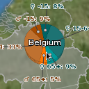
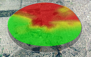
Lightspeed: Highlighting samples.lightspeed.customization.style.highlighting.MainPanel
This sample demonstrates how LuciadLightspeed's animation and style frameworks can be used to highlight and show custom animations for the object under the cursor.
The sample consists of a layer containing shapes for each country. When the mouse is moved over a country, a pie chart appears showing the demographic distribution in that country.
This layer has two stylers:
- An
AnimatedHighlightAreaShapeStylerwhich takes care of the styling of the countries/pie charts themselves ( fill/line colors ) - An
AnimatedHighlightAreaLabelStylerwhich takes care of the styling of the labels of the countries/pie charts
ALcdAnimationManager
and
ALcdAnimation
in combination with a mouse
adapter to progressively adjust the styles of each object.
The pie charts are created and styled by passing their style and geometry to a
ALspStyleCollector
along with the object to which they belong.
Instructions
Move your cursor over the different countries of the world. When the cursor is on top of a country, a pie chart will gradually rise and display population statistics specific of that country. When the cursor moves away from the highlighted country, the pie chart for that country will gradually vanish.
Lightspeed: Thematic mapping samples.lightspeed.customization.style.thematic.MainPanel
This sample demonstrates how to implement "thematic mapping", i.e. to adjust the style of an object to that object's attributes.
The sample consists of a layer of country shapes on which custom colors are being styled.
The colors for the countries are linearly interpolated between a minimum color and a maximum color
chosen by the user, with the population of each country as a weight for the interpolation.
More populated areas will therefore tend towards the maximum color, while less populated
areas will tend towards the minimum color. This styling is accomplished by using a custom
styler implementation, namely a
samples.lightspeed.customization.style.thematic.CountryStyler
Instructions
Click on either the left or right gradient button on the toolbar to set the lowest or highest population color respectively. You will notice that the color of the countries is an interpolated value between those two colors, based on their population.
Data Model Tree Sample samples.lightspeed.datamodel.MainPanel
This sample adds functionality to view the TLcdDataModel of an ILcdModel that has an ILcdDataModelDescriptor as a model descriptor.
The 'Data Model Tree' is visible on start-up, showing the data model tree for the currently selected layer.
The data model tree contains all declared TLcdDataType instances of the TLcdDataModel. Each TLcdDataType contains a series of properties and TLcdDataProperties.
All TLcdDataTypes that are also model element TLcdDataType instances are highlighted in a special color.
Note that TLcdDataModel instances can define data types that are cyclical. There is no explicit check for this issue in the sample code, as it was not needed for this special case.
Instructions
Open some random files and see how the data model tree gets updated each time you select a new layer which has an ILcdModelDescriptor as model descriptor on its model.
Lightspeed: Day/night Map samples.lightspeed.daynight.MainPanel
This sample shows how to create a day/night map in a Lightspeed view. The areas in civil/nautical/astronomical twilight and night are drawn in progressively darker shades. An icon on the map indicates the point where the sun is directly overhead. The day/night map animates in fast time over a period of 1 year.
The day/night map is constructed as follows:
- Find the point on the Earth where the sun is directly overhead.
- On the opposite side of the globe, construct a set of concentric circles to represent the night and twilight areas.
- Fill these circles with a dark translucent color.
Instructions
The sample automatically shows an animated day/night map. A label on the top edge of the map shows the current date and time of the map.
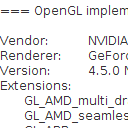
Lightspeed: Hardware capability report samples.lightspeed.debug.report.MainPanel
The hardware capability report sample generates a detailed list of the hardware related
capabilities of the device running the sample. The sample generates a hardware
report with the OpenGL and OpenCL capabilities of the system using the
com.luciad.view.lightspeed.util.TLspPlatformInfo
utility class.
Reported capabilities include:
- OS information
- OpenGL basic information (vendor, renderer, version)
- OpenGL available extensions
- OpenGL state variables
- OpenCL basic information (vendor, version, ...)
- OpenCL available extensions
- OpenCL device info
Instructions
When contacting Luciad support about any Lightspeed-related problems, it is always appreciated if you include the report generated by this sample.
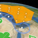
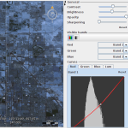
Lightspeed: Decoding multiple format data samples.lightspeed.decoder.MainPanel
This sample demonstrates the ability to load and visualize data from sources in different formats
on a Lightspeed map using ILcdModelDecoder and ILspLayerFactory.
A File and a URL action are configured to load data in almost every available format.
The sample uses a composite ILcdModelDecoder to decode the data into anILcdModel.
After this, a composite ILspLayerFactory creates a layer that controls how
the model of the loaded data is displayed.
The model decoders and layer factories are retrieved using a service look-up mechanism, and
contain both built-in and sample implementations.
The toolbar includes several controllers to visually compare layers.
Instructions
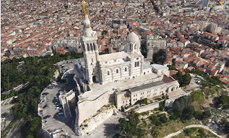
Add new data by pressing the appropriate toolbar button or by dragging and dropping files or URLs on the map. Not all styled LuciadLightspeed formats have a dedicated Lightspeed layer factory (an example of this is DGN), in which case a fallback layer factory is used. As a result, the visualization of some data might not be correctly styled. The data shown in the highlighted sample screenshot is an OGC 3D Tiles mesh data set for Marseille, located at https://sampleservices.luciad.com/ogc/3dtiles/marseille-mesh/tileset.json.
The toolbar allows selecting the following visual inspection controllers:
- The swipe controller: Select two sets of layers. Drag the swipe line horizontally or vertically to inspect differences between the two sets along the line.
- The flicker controller: Select two layers. Quickly click the mouse to toggle between the two layers.
- The porthole controller: Select two sets of layers and move your mouse over the map. The first set of layers is visible by default. The second set is shown in a rectangular area around the mouse location. Holding down the shift key and moving the mouse wheel resizes the porthole.
- The magnifier controller: a square area around the mouse location shows a zoomed in view of the visible layers. In the magnifier overlay, view-sized items still have the same size while world-sized items are scaled to respect the zoom-factor of the magnifier. Holding down the shift key and moving the mouse wheel changes the zoom factor of the magnifier. Holding down the control key and moving the mouse wheel resizes the magnifier overlay.
Lightspeed: Editing geometric shapes samples.lightspeed.editing.MainPanel
This sample illustrates the editing and creation capabilities of the editors that are available in the Lightspeed API. The sample contains one shape layer for both editing and creation. Shape creation is performed using TLspCreateController. Shape editing is performed using TLspEditController.
Consult the developer's guide or the documented source code of this sample for detailed information on how to create an application that uses Lightspeed editors.
Instructions
To edit one of the shapes, click on the shape and interact with one of its edit handles. Please refer to the javadoc of the different editor classes in the com.luciad.view.lightspeed.editor package to see what functionality is provided by each of the handles.
To create a new shape, activate one of the create controllers in the toolbar. Most of the controllers also have an extruded creation variant. This variant creates an extruded shape with the base shape that is created by the normal editor. For instance, the ellipse create controller creates an extruded ellipse when extrusion is activated. Extrusion can be activated by the extrusion button in the creation toolbar.
For most shapes creation is simply performed by a sequence of mouse clicks or taps. Some additional instructions for special cases:
- Polylines and polygons: End creation by right or double clicking.
- Complex polygons: Advance to the next polygon by right clicking. Finalize the creation process by double clicking.
- Complex rings and curves: Advance to the next shape by right clicking. Change the shape type using one of the buttons that appear in the view.
- Extruded polylines and polygons: End creation of the base shape by right clicking.
When creating or editing shapes you can disable snapping by pressing the control key (cmd on macOS). Insert or remove a point from a polyline or polygon by holding down the control key (cmd on macOS) while pressing. Select multiple shapes by holding the shift while pressing. Use the delete key to remove selected shapes.
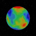
Lightspeed: Geoid samples.lightspeed.geoid.MainPanel
This sample visualizes the EGM2008 geoid in 3D. The geoid heights are exaggerated; they actually vary between -110m and +90m. Blue colors indicate that the geoid heights are negative (geoid below the ellipsoid of the WGS84 datum). Green colors indicate that the geoid heights are positive (geoid above the ellipsoid).
Geoid heights are typically used behind the screens, in calculations with references that have geodetic datums based on geoids. They are relevant for elevation data, for instance, which are commonly defined with respect to a few standardized geoid models. For accurate computations, elevations above a geoid can then be transformed to elevations above an ellipsoid.
The geoid heights are retrieved from the geodetic datum that is created by the TLcdGeoidGeodeticDatumFactory.
Instructions

Lightspeed: Grids samples.lightspeed.grid.MainPanel
This sample demonstrates how to display grid layers in a Lightspeed view.
The following grid layers are included:
- Lon Lat: a simple multi-level grid showing longitude and latitude lines. The lines are refined up to the second.
- Georef: an alphanumeric multi-level grid based on longitude latitude lines. The lines are refined up to the degree. The labels denote 1-by-1 degree squares.
- XY: a grid based on an ILcdXYWorldReference. The labels denote meters.
In addition, the sample shows how to change text and line styles and other grid styling properties.
Instructions
- Select a grid type and an appropriate projection
- Pan and zoom around. Notice how the grid and its labels adapt.
- Change some styling options. The results are shown instantly.
Lightspeed: 3D icons samples.lightspeed.icons3d.MainPanel
This sample demonstrates how to visualize point data using 3D icons. Icons can be loaded from files in either Collada, OpenFlight or WaveFront OBJ format.
Instructions
The sample shows animated 3D points. At startup, they are displayed using an airplane icon. Use the "open" button on the toolbar to load a .DAE, .OBJ or .FLT file. Doing so will replace the airplane model.
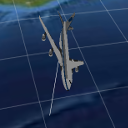
Lightspeed: Image Projection samples.lightspeed.imageprojection.MainPanel
This sample demonstrates how to project images on terrain.
Instructions
The sample shows an image being projected on terrain by an animated plane. Notice how the projected image deforms when projected on the terrain. The white lines indicate the projection frustum. This frustum can be toggled on or off in the layer pane.
Lightspeed: Multispectral image visualization samples.lightspeed.imaging.multispectral.MainPanel
This sample illustrates how multispectral raster imagery can be visualized and analyzed in an ILspView.
The sample starts with pre-loaded satellite image files covering the region of Las Vegas. The images are obtained from the LandSat7 USGS archive. They are multi-spectral GeoTIFF files that consist of 7 bands. The sample also allows you to load other GeoTIFF files from disk.
The panel below the layer controls demonstrates the LuciadLightspeed imaging operators and filters, and allows you to configure how the image in the selected layer is displayed. You can adjust brightness, contrast, opacity, and apply a sharpening filter using the sliders.
You can also choose which of the 7 image bands are displayed, and to which color channel they are mapped. To display the pre-loaded images in the the LandSat7 natural color preset for instance, select the bands 3, 2 and 1 in the Red, Green and Blue drop-down menus respectively. Other interesting band combinations that highlight specific aspects of the image data are 4-3-2, to display the near infrared (NIR) data, and 7-4-2 to display short-wavelength infrared (SWIR) data. The band combination 7-4-2 displays vegetation in bright shades of green, for instance.
The Curves panel displays the data distribution of the displayed image bands in a histogram. You can adjust the dynamic range for the bands in each color channel by manipulating the line displayed on top of the histogram into a curve. You can also enhance the image contrast automatically by applying the Equalization function on the Luminance tab.
The toolbar allows selecting a swipe and flicker controller to visually compare layers.The swipe controller displays a swipe line that can be dragged horizontally or vertically, displaying only half of the first set of layers on the left or top side, and half of the other set of layers on the other side. The flicker controller allows to quickly toggle between multiple layer sets by clicking the mouse. See the documentation of TLspSwipeController and TLspFlickerController for more info.
The sample makes use of TLspImageFilterStyle and the ALcdImageOperator API to perform the band selection and dynamic range adjustments.
Instructions
Load additional files with drag and drop, or by clicking the Open button on the toolbar. When you select the resulting layer in the layer control panel, three additional panels appear below the layer controls.
In the General panel, you can apply several image filters to the selected raster layer. Use the sliders to adapt the image contrast, brightness, opacity and sharpness.Click Reset to return to the default filter settings.
The Visible bands panel allows you to choose which image bands are made visible, and in which color. The drop-down
menus next to the Red, Green and Blue color channels contain a list of the image bands present in the
selected raster layer. To map an image band to a particular color channel, select the band number from the
drop-down menu next to the preferred color.
To see just one band in grayscale, click the grayscale icon and select a band from the drop-down menu.
The Curves panel consists of four tabs. The Red, Green and Blue tabs displays a histogram and a tone curve for the
color-mapped bands of the loaded image. To see the histogram and tone curve for a particular band, select the tab
with the color to which you mapped the band. To change the tone curve in a particular color channel, select the
line on the histogram, and drag its control points until it forms a curve, and your image displays the required
color balance. You can add or delete points on the selected curve by ctrl-clicking. The Luminance tab displays
a histogram and curve for the brightness of the image. You can manipulate the tone curve to improve the contrast
in the image. To enhance image contrast automatically, click Equalize. As a result, the contrast will be
stretched automatically, and the curve will change.
To reset curves to their original settings, click Reset.
To visually compare layers, select the swipe controller from the toolbar. Compare for example the Las Vegas image from 2000 and 2003. By dragging the swipe line you should be able to easily see the differences between the two image files. Enable the flicker controller from the toolbar and select the two Las Vegas image files. Quickly click the mouse to toggle between the two layers.
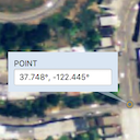
Lightspeed (JavaFX): Balloon samples.lightspeed.javafx.balloon.Main
This sample demonstrates how to display balloons in a TLspFXView using TLspFXBalloonManager.
This sample requires JavaFX. Depending on the JDK you are using, you may need to install it separately.
Refer to the technical notes in the documentation for more information.
The sample shows two points on the map, each of which is tied to a balloon. A balloon is made visible when a single object is selected. The balloon contains an editable text field containing the position of the icon in geodetic coordinates.
For a more extensive description of the balloon manager API see the developers' guide.
Instructions
Select one of the icons. A balloon will appear. Editing the coordinate panel in the balloon and hitting return will change the location of the icon. The balloon arrow also gets relocated with this operation. Balloons are only shown when one domain object is selected.
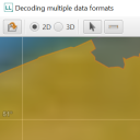
Lightspeed (JavaFX): Decoding multiple format data samples.lightspeed.javafx.decoder.Main
This sample demonstrates the ability to load, visualize and print data from sources in different formats
on a Lightspeed JavaFX map using ILcdModelDecoder and ILspLayerFactory.
This sample requires JavaFX. Depending on the JDK you are using, you may need to install it separately.
Refer to the technical notes in the documentation for more information.
A file and a URL action are configured to load data in almost every available format.
The sample uses a composite ILcdModelDecoder to decode the data into anILcdModel.
After this, a composite ILspLayerFactory creates a layer that controls how
the model of the loaded data is displayed.
The model decoders and layer factories are retrieved using a service look-up mechanism, and
contain both built-in and sample implementations.
Instructions
Add new data by pressing the appropriate toolbar button or by dragging and dropping files or URLs on the map. Not all styled LuciadLightspeed formats have a dedicated Lightspeed layer factory (an example of this is DGN), in which case a fallback layer factory is used. As a result, the visualization of some data might not be correctly styled.
Use the print button on the toolbar to preview and print the current contents of the map.

Lightspeed (JavaFX): Editing geometric shapes samples.lightspeed.javafx.editing.Main
This sample illustrates the editing and creation capabilities of the editors that are available in the Lightspeed API.
This sample requires JavaFX. Depending on the JDK you are using, you may need to install it separately.
Refer to the technical notes in the documentation for more information.
The sample contains one shape layer for both editing and creation. Shape creation is performed using TLspCreateController. Shape editing is performed using TLspEditController.
Consult the developer's guide or the documented source code of this sample for detailed information on how to create an application that uses Lightspeed editors.
Instructions
To edit one of the shapes, click on the shape and interact with one of its edit handles. Please refer to the javadoc of the different editor classes in the com.luciad.view.lightspeed.editor package to see what functionality is provided by each of the handles.
To create a new shape, activate one of the create controllers in the toolbar. Most of the controllers also have an extruded creation variant. This variant creates an extruded shape with the base shape that is created by the normal editor. For instance, the ellipse create controller creates an extruded ellipse when extrusion is activated. Extrusion can be activated by the extrusion button in the creation toolbar.
For most shapes creation is simply performed by a sequence of mouse clicks or taps. Some additional instructions for special cases:
- Polylines and polygons: End creation by right or double clicking.
- Complex polygons: Advance to the next polygon by right clicking. Finalize the creation process by double clicking.
- Complex rings and curves: Advance to the next shape by right clicking. Change the shape type using one of the buttons that appear in the view.
- Extruded polylines and polygons: End creation of the base shape by right clicking.
When creating or editing shapes you can disable snapping by pressing the control key (cmd on macOS). Insert or remove a point from a polyline or polygon by holding down the control key (cmd on macOS) while pressing. Select multiple shapes by holding the shift while pressing. Use the delete key to remove selected shapes.
Lightspeed: JavaFX touch editing samples.lightspeed.javafx.touch.Main
This sample demonstrates how to add touch support into a JavaFX application.
This sample requires JavaFX. Depending on the JDK you are using, you may need to install it separately.
Refer to the technical notes in the documentation for more information.
The sample features large buttons to allow easy manipulation with fingers instead of a mouse as input device.
Instructions
Use one finger to pan around and to select or edit objects. Use two fingers to zoom or rotate.
To edit one of the shapes, you just have to touch the shape and interact with one of its editing handles. Please refer to the javadoc of the different editor classes in the API to see what functionality is provided by each of the handles.
To create a new shape, activate one of the create controllers in the toolbar. Note that most of the controllers also have an extruded creation variant. This variant creates an extruded shape with the base shape that is created by the normal editor. For instance, the ellipse create controller creates an extruded ellipse when extrusion is activated. Extrusion can be activated by the extrusion button in the creation toolbar (third button).
Some shapes like polylines, polygons, and complex polygons have different (dynamic) creation steps that can be ended by pressing the Commit button. For example, to create a complex polygon containing two triangular shapes, the sequence of interactions should be: tap-tap-tap, commit (to end first polygon), tap-tap-tap, commit (to end second polygon), commit (to end complex polygon creation).
Lightspeed: Interactive labels samples.lightspeed.labels.interactive.MainPanel
This sample demonstrates how labels can be made editable. The labels are editable in the sense that they can be moved to a new location, as well as in the sense that they offer the user an interactive component that can be used to edit information related to the domain objects.
Instructions
Move the mouse over a label of a city. An interactive, editable label will be shown instead of the regular label. You can enter a comment for the labeled city in the text field. To apply the changes, press the Enter key or press the green tick mark at the top of the interactive label. To cancel the outstanding changes, press the red 'cancel' icon at the top of the label or press the Escape key.
The interactive label can be moved by clicking and dragging on the title bar of the interactive label.
Lightspeed: Label placement samples.lightspeed.labels.placement.MainPanel
This sample demonstrates various labeling algorithms:
- TLspLabelingAlgorithm, for labeling cities
- TLspInPathLabelingAlgorithm, for labeling states
- TLspCurvedPathLabelingAlgorithm, for labeling rivers
Note that the river's springs are determined as the first point of the first polyline, which may not correspond to reality.
Instructions
To see the effects of the labeling algorithms select a layer, by clicking it in the layer control and:
- change the layer's visibility
- set the layer labeled/not labeled
- move the layer up/down: labeling is started from the topmost layer
To modify the label styling, drag the opacity slider, or change the font using the Font combobox.
Lightspeed: Lightweight views samples.lightspeed.lightweight.MainPanel
This sample demonstrates how Swing components can be overlaid on an ILspView. Specifically, the sample shows a JInternalFrame which contains a secondary map view, alongside with navigation controls for the main view.
To avoid issues with the mixing of lightweight and heavyweight components, the sample uses TLspSwingView rather than TLspAWTView. A JLayeredPane is added to the main view. Within this layered pane, one layer is a JDesktopPane containing the internal frame with the second view. Another layer contains the standard navigation controls and scale indicator for the main view (as can also be seen in other samples).
Instructions
Move, resize, minimize and maximize the internal frame. Observe how it sits between the main view and its overlaid navigation controls.
Lightspeed: Constrained navigation samples.lightspeed.limitnavigation.MainPanel
This sample demonstrates how the view-world transformation can be customized in order to constrain the navigation freedom. This behavior can be enabled or disabled using a checkbox in the toolbar.
Instructions
Take note of the checkbox labeled "Limit Navigation" in the upper right corner of the screen, by default it is checked. As long as this checkbox is checked your navigational options are constrained:
- Rotate the view, notice how this has no effect. The view is automatically rotated to keep the north at the top of the screen.
- Zoom in and out, notice how you can only zoom out to a certain degree and how you can only zoom in to a certain degree and only to a certain area marked by the red rectangle.
- Pan and navigate around the view, notice how you can only pan to the boundaries of the area marked by the red rectangle.
Uncheck the "Limit Navigation" checkbox and retry panning, zooming and rotating the view and notice the difference with the constrained version of these behaviors.
Lightspeed: Map Overview samples.lightspeed.mapoverview.MainPanel
This sample shows to add a map overview for an ILspView. The map overview is overlaid on the main view. It shows the bounds of the area of the world that is visible in the main view.
The map overview is itself a TLspSwingView, which is added to the main view's overlay panel. The visible map area is obtained using ALspViewXYZWorldTransformation.getGeodeticVisibleArea(). The map overview continuously fits to this polygon.
Instructions
Navigate in the main view. Switch between 3D and the various 2D projections. Observe how the map overview updates continuously and how the polygon in the map overview corresponds to the area of the world that can be seen in the main view.
Lightspeed: Encode shape as JSON mesh samples.lightspeed.meshencoder.MainPanel
This sample demonstrates how 3D shapes in LuciadLightspeed can be discretized and saved as 3D meshes in a custom file format.
The intent of this sample is to show you how to export 3D shapes from LuciadLightspeed as 3D meshes for re-use in a LuciadRIA client. The produced JSON file can easily be parsed by the LuciadRIA MeshFactory.
Instructions
To save a 3D shape as a JSON mesh-file, select a shape in the view, and press the save button in the toolbar.
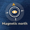
Lightspeed: Navigation controls samples.lightspeed.navigationcontrols.MainPanel
This sample demonstrates how to use
TLspNavigationControlsFactory
to create
Swing-based controls for view navigation and overlay these controls on a view.
The default navigation controls are as usual visible in the top right corner. A secondary set of controls is added to the left side of the view. The distinct components are the same but they are separated and added in different corners and they always appear active. The compass navigation control on the left side points towards the magnetic north instead of the real north.
Instructions
Use the secondary set of navigation controls to pan, zoom and rotate the view.
Lightspeed: Painting data that is not geographically referenced samples.lightspeed.nongeoreferenced.MainPanel
This sample contains three layers:
- Raster data: a GIF file of Washington DC.
- Vector data: a number of vector shapes drawn on top of the raster.
- XY Grid: an xy grid, including labels.
Instructions
Navigate the map. Notice how the mouse location at the bottom indicates the pixel coordinates in the image.
Select one of the shapes and edit it or create a new shape.
Open an image file.
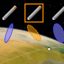
Lightspeed: Painting in view coordinates samples.lightspeed.paintinview.MainPanel
This sample contains two layers:
- Screen data: a point, polygon and ellipse defined in screen coordinates. This is achieved by using a model reference that is not an ILcdGeoReference.
- Georeferenced data: three lon-lat ellipses. For each ellipse, a pencil icon is drawn in screen coordinates, as well as a mini version of the ellipse. This is achieved by using an ALspStyleTargetProvider that returns null as its target geo reference.
Instructions
Navigate the map. Notice how the shapes at the top of the screen remain at the same position at any time.
Select one of the green shapes and edit it.
Select one of the blue ellipses. One of the icons and mini-ellipses is automatically selected as well.
Select one of the pencil icons or mini-ellipse. The corresponding ellipse is selected as well.
Edit one of the blue ellipses. The corresponding mini-ellipse is edited as well.
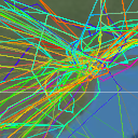
Lightspeed: Plot painting samples.lightspeed.plots.MainPanel
The sample loads 500.000 aircraft positions around New York.
The plots are painted with a plot layer (TLspPlotLayerBuilder).
At a certain scale, heading arrows are displayed, and labels that are de-cluttered using the continuous de-cluttering algorithm.
Filtering can be done through the properties of the data model.
- Ranged properties (such as time, speed) can be filtered using the sliders
- For properties with limited values (such as class) you can select one value from the drop-down boxes
Styling is also based on the properties of the data model.
- For ranged properties (such as time, speed) the icon color is interpolated between red and green based on the filter sliders
- For properties with limited values (such as class) a color or icon is automatically assigned to each possible value
Instructions
Change the filtering through the sliders and drop-down boxes. The filter is immediately effective.
Change the color and icons through the drop-down boxes. The change is immediately effective.
Enable and disable density plots through the checkbox. The change is immediately effective.
Lightspeed: Printing samples.lightspeed.printing.MainPanel
This sample demonstrates how to print a component containing a view, using the TLspViewComponentPrintable.
Instructions
The sample creates a page layout containing the view and some decorations. You can preview the page or print it directly using the buttons in the toolbar.
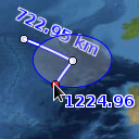
Lightspeed: Measurement Controller samples.lightspeed.ruler.MainPanel
This sample demonstrates how to configure the measurement controller and change different properties of it dynamically at runtime.
Instructions
It is possible to modify the following ruler settings:
- Measure mode: Geodetic, Rhumbline or Cartesian. The latter measures cartesian distances between points in world coordinates, which is useful e.g. to measure the height of a 3D shape.
- Color style: the color of the measurement polylines.
- Font style: the font of the labels.
- Distance unit: Meters, Kilometers, Feet or US Miles.
- Display azimuth: the azimuth of the measurement segments.
- Display Equal Distance Circles: visual aid during editing of measurements. Only supported in the Geodetic measure mode.
- Keep Measurements: Don't delete the old measurement when starting the creation of a new one.
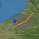
Lightspeed: Displaying shapes samples.lightspeed.shapes.MainPanel
This sample shows how to programmatically create and display a model. It reveals how to create an ILcdModel, how to populate it with ILcdShape objects, and how to display that data in an ILspLayer on a Lightspeed view.
For a more extensive description of each of these steps see the developers' guide.
Instructions
The sample shows a polyline, a polygon, and a point visualized by an icon. Try interacting with the shapes.
Lightspeed: Editing the style of objects samples.lightspeed.style.editable.MainPanel
This sample is intended to illustrate the process of editing an object's style at runtime.
It creates a setup in which a
TLspEditableStyler
is used to edit the
styles of all the objects. To tweak the values of the provider at runtime, a widget was
implemented which provides a GUI for editing the most prominent style properties (see
StyleEditor
andStyleEditorModel).
Note that for simplicity, this sample focuses on editing line- and fill styles, but the concepts used in this sample can be applied to editing other styles as well.
Instructions
- Select an object in the view.
- Press the edit style button in the toolbar.
- In the style dialog that appears, change the desired settings.
- Press "OK" to apply the new settings and close the dialog (if you just want to apply the settings and keep the dialog open, press "Apply").
- Line Width: use the spinner widget to change the line width.
- Line Color: click on the color label to choose a different color.
- Line Pattern: choose a different line pattern from the drop down.
- Fill Color: click on the color label to choose a different color.
- Fill Pattern: choose a different fill pattern from the drop down.
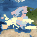
Lightspeed: Expression-based styling of objects samples.lightspeed.style.expressions.MainPanel
This sample demonstrates expression based-styling in a Lightspeed view using
TLspParameterizedLineStyle, TLspParameterizedFillStyle and
TLspParameterizedIconStyle
Instructions
Use the layer selection panel on the right to select different layers, demonstrating different kinds parameterized
styles, ILcdExpression and shapes.
The first layer shows Flightradar tracks styled with a TLspParameterizedLineStyle. Only the segment
of a track that is within a specified time interval is visible.
The second layer shows European countries styled with a TLspParameterizedFillStyle. The fill color
of the countries is derived from the population property of each country.
The last layer visualizes cities using a TLspParameterizedIconStyle. An icon for a city is scaled based
on the population property and the distance to the mouse cursor.
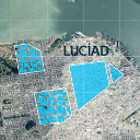
Lightspeed: Fill style samples.lightspeed.style.fillstyle.MainPanel
This sample demonstrates the capabilities of TLspFillStyle. It shows various layers with
shapes with different fill styles:
- Solid: the area is filled with one color, possibly transparent.
- Stippled:
the area is filled with a repeating pattern. A stipple pattern is created by using
a
TLspFillStyle.StipplePatternwith convenience methods to draw lines or filled/outlined rectangles, ovals or polygons. - Textured:
the area is filled based on an texture. This can be a
BufferedImage, and can be scaled, rotated or translated. Additionally, the texture can be set to be applied relative to the bounds of the object or relative to the bounds of the world.
Instructions
The sample has various layers containing shapes with different fill styles.
Move around in 2D and 3D to see the effect.
Edit the shapes to see how the different fill styles adapt.
Lightspeed: Icon style samples.lightspeed.style.icon.MainPanel
The icon style sample demonstrates the icon styling functionality of TLspShapeLayerBuilder, i.e.: rotation and transparency of icons, drawing icons with a vertical line and drawing icons either with a size in world coordinates or in view coordinates. All this is accomplished using TLspIconStyle.
The sample contains three layers with icons, all located around San Francisco:
- View sized icons: the icon size remains constant in view coordinates (i.e. pixels), regardless of the scale of the view.
- World sized icons: the size of the icons remains constant in world coordinates (typically meters).
- Rotatable icons: these icons use a custom styler (see RotatableIconStyler). They can be rotated using the slider in the upper left corner of the view. They also change color depending on the scale of the view. Finally, the icons use a third scaling mode which is a hybrid of view and world sized: the size of the icons is defined in world coordinates, but their size on screen will never exceed their native size in pixels.
Instructions
Zoom in on San Francisco and see how each icon layer resizes its icons differently. Also notice how the rotatable icons layer changes the color of its icons based on the scale of the view. Use the rotation slider to change the orientation of the rotatable icons.
Lightspeed: Raster style samples.lightspeed.style.raster.MainPanel
The Raster Style sample illustrates how the style of a raster can be changed on the fly:
- Change the outline and fill of the raster's bounds.
- Change brightness, contrast and opacity.
- Set and change a custom filter (interactive raster layers only).
- Change the color model for elevation layers.
The sample starts with a raster style with 100% brightness, 100% contrast, 100% opacity and no custom filter. For more detailed information on how to use raster styles and providers, see the developer's guide or the documented source code of this sample.
The sample shows 3 types of layers:
- Interactive raster layers: the style of these layers can be changed interactively. They are marked with a [I] prefix.
- Background raster layers: the style of these layers can be changed but not as smoothly as interactive layers. However they generally require less processing and memory for painting. These layers are marked with a [B] prefix.
- Terrain layer: this layer is a proxy for the view's terrain. The view's terrain contains all background layers at the bottom of the view, hence changing its style will affect all those layers. Its style can be changed interactively.
Instructions
Select a raster layer in the layer control and change its style using the panel on the left.
Lightspeed: Stroked line styles samples.lightspeed.style.strokedline.MainPanel
This sample demonstrates how line data can be visualized using complex strokes. This is achieved by using TLspComplexStrokedLineStyle.
Instructions
The sample shows a number of shapes with different strokes. Use the layer selection panel on the right to select different layers, demonstrating different kinds of strokes. Select and edit the shapes to see how the stroke pattern adjusts itself. Switch to a 3D view to see how stroked lines appear when they are draped over the terrain.
Lightspeed: Touch Basic samples.lightspeed.touch.basic.MainPanel
This applet demonstrates the use of the touch-based ILspControllers.
It features a single controller chain to navigate around the map, and select and edit objects.
The sample features large buttons to allow easy manipulation with fingers instead of a mouse as input device.
Instructions
Use one finger to pan around and to select or edit objects. Use two fingers to zoom.
Lightspeed: Custom touch controller samples.lightspeed.touch.customcontroller.MainPanel
This sample demonstrates how ALspController can be extended to implement a custom
touch controller.
The first custom controller displays a tooltip for objects that are touched.
The second custom controller fits the view to the bounds of an object if a touch-and-hold action is performed on that object.
Instructions
Activate the first custom controller ("information panels"). While you touch an object on the map (e.g. a county), a tooltip will pop up showing some of that object's attributes.
Activate the second custom controller ("fit to object"). Touch and hold an object until a red circle visually notifies you that the touch-and-hold time has been reached. If you now release your finger, the view will fit to the bounds of that object.
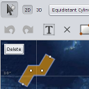
Lightspeed: Touch Editing samples.lightspeed.touch.editing.MainPanel
This applet demonstrates the use of the touch-based ILspControllers for editing purposes.
Instructions
Navigate, select and edit objects. You can make a layer selectable by first tapping on its name in the layer list, and then tapping on the "Toggle layer selectable" button.
To edit one of the shapes, you just have to touch the shape and interact with one of its editing handles. Please refer to the javadoc of the different editor classes in the API to see what functionality is provided by each of the handles.
To create a new shape, activate one of the create controllers in the toolbar. Note that most of the controllers also have an extruded creation variant. This variant creates an extruded shape with the base shape that is created by the normal editor. For instance, the ellipse create controller creates an extruded ellipse when extrusion is activated. Extrusion can be activated by the extrusion button in the creation toolbar (right most button).
Some shapes like polylines, polygons, and complex polygons have different (dynamic) creation steps that can be ended by pressing the Commit button. For example, to create a complex polygon containing two triangular shapes, the sequence of interactions should be: tap-tap-tap, commit (to end first polygon), tap-tap-tap, commit (to end second polygon), commit (to end complex polygon creation).

Lightspeed: Simulation of touch events samples.lightspeed.touch.touchEvents.MainPanel
This sample demonstrates the effect of touch events on a touch enabled Lightspeed view. It contains a setup that simulates touch events and passes them to the Lightspeed view. The touch controller set on the view is a navigation controller by default and will interpret the incoming events by panning and zooming the view.
The simulation can be started by clicking the "Simulate touch events" button in the toolbar.
Instructions
Start a simulation of how touch events are handled in a Lightspeed view by clicking the button in the toolbar.
Lightspeed: Tracking camera samples.lightspeed.trackingcamera.MainPanel
This sample shows how different constraints can be added to the view's camera to automatically follow one or more moving objects.
The sample shows a model with three airplanes. Their position is constantly updated. The sample attaches a tracking constraint to the camera so the airplanes are always in view.
The different possible tracking constraints are:
TLspLookFromTrackingCameraConstraint3D: used to fix the camera at a certain position. Panning and zooming are not possible, but rotating still is. Optionally, the direction of the camera can be fixed as well, so rotating is also impossible.TLspLookAtTrackingCameraConstraint3D: used to fix the camera in a certain direction. Panning is not possible, but zooming and rotating still is.TLspLookAtTrackingCameraConstraint2D: same as above for 2D views.
Instructions
The combobox on the right shows the available tracking modes. It changes the world reference, view's camera, and the tracking mode.
Supported tracking modes for a 3D view are:
- Look at target: the camera is always oriented towards the tracked objects. Panning is not possible, but zooming and rotating is.
- Look from target: the camera is always positioned on the tracked objects, looking away from them. Panning and zooming are not possible, but rotating is.
- Oriented like target: the camera is always positioned on the tracked objects, oriented like the objects (based on ILcdOriented). Panning, zooming and rotating is impossible.
- Follow location: the camera is always oriented towards the tracked objects. Panning is not possible, but zooming and rotating is.
- Follow location and orientation: the camera is always positioned on the tracked objects, oriented like the objects. Only zooming is possible.
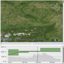
Lightspeed: Vertical view samples.lightspeed.vertical.MainPanel
This sample demonstrates the use of the vertical view package. The 2D view in the upper part contains a flight layer with two flight routes. Each flight route is modeled as a list of 3D points.
The vertical view in the lower part is used to display the vertical profile of the flight that is selected in the 2D view. Apart from this profile, a number of sub-profiles associated to it can be shown in a vertical view. In this case, two sub-profiles are associated to the view: the terrain and the air route. FlightVVModel, an implementation of ILcdVVModel holds the main-profile points and the information about the sub-profile.
Instructions
Select a flight. A vertical marker is shown in both views. Change the height of the flight by dragging its points up or down. You can zoom the X and Y axes by using the sliders to the right and at the bottom. You can disregard flight points at the left or right of the flight using the sliders at the top. Finally, the panel at the right allows you to select the altitude unit.
Lightspeed: style layers using Symbology Encoding (SLD) samples.ogc.sld.lightspeed.MainPanel
The OGC Symbology Encoding (Styled Layer Descriptor) standard describes an XML format to describe the style of a layer. This sample demonstrates how to decode such a style from a file and how to apply it to a Lightspeed layer.
The application displays a number of layers and a set of styles. The styles can be applied to the layers. Some of the styles are specific for a particular layer, while others can be applied to any layer.
The text area at the right displays the description of the style as it is defined in the SLD file.
Instructions
Select a layer in the layer control and a style in the dropdown list. Selecting the style will automatically apply it to the selected layer.
Decoding ISO19139 metadata samples.metadata.MainPanel
This sample demonstrates the ability to load metadata encoded following the ISO 19139 standard schema.
Instructions
Click the open button and select a file from the LuciadLightspeed/samples/resources/Data/metadata folder. The central frame will display the metadata as encoded in the file.
Metadata gazetteer samples.metadata.gazetteer.MainPanel
This sample demonstrates a simple gazetteer functionality.
Some metadata files are loaded and the geographic extent of the data they describe is extracted from the metadata and displayed on the map as bounds.
Instructions
Double click on the bounds to display all metadata linked to the bounds.
Right click with the mouse to load the data which is described in the metadata. The location(s) of the file to load is extracted from the metadata.
GXY: Displaying dynamic data samples.realtime.gxy.tracksimulator.MainPanel
This sample shows how to visualize dynamic tracks in a GXY map.
The sample shows several random parabolic trajectories and animates 2000 dynamic tracks moving
along these trajectories. The dynamic tracks layer is simulated using a
TLcdSimulator with a custom ALcdSimulatorModel.
Each track has a label that displays its identifier, and the grounded state of the track.
Instructions
Press the "Play" button to start or the simulation. The tracks start moving across their individual trajectories.
As the tracks move around, the labels are gently repositioned to avoid overlap. If you hover the mouse over a label of a moving track, it stops moving. In the rare event labels get mixed up, you drag them to a new location. Labels move back automatically.
A time slider allows to see your progression in the simulation. When the simulation is not running, the slider also allows you to change the "simulation time" with your mouse.
You can adjust the replay speed factor using the "speed up" slider.

Lightspeed: Displaying dynamic data on a map and timeline samples.realtime.lightspeed.tracksimulator.MainPanel
This sample shows how to visualize dynamic tracks in a Lightspeed map and timeline.
The sample shows 2000 random parabolic trajectories and animates 2000 dynamic tracks moving
along these trajectories. The dynamic tracks layer is simulated using a
TLcdSimulator with a custom ALcdSimulatorModel.
Tracks are visualized with airplane icons. In 3D projections, a line connects each icon with its zero-elevation
point.
Each track also has a trail of grey dots indicating previous positions. The trail is added to
the icons by using a custom ILspStyler.
The track labels are decluttered using the TLspContinuousLabelingAlgorithm,
a specialized algorithm for moving objects in a Lightspeed view.
The time line at the bottom is a non geo-referenced Lightspeed view that you can pan and zoom.
Instructions
Press the "Play" button to start the simulation. The tracks start moving across their individual trajectories. The time view is also updated. If you pan the time view, the simulation is also updated. You can adjust the replay speed by zooming in or out on the time line.
Select a plane in the main view. Its altitude over time is displayed in the time view along with the name of its landing and take-off city.
Zoom in and pan around the world to see how the labels of the dynamic tracks are automatically decluttered depending on the current situation. You can also select and move all of the track labels.
GXY: style layers using SymbologyEncoding (SLD) samples.ogc.sld.gxy.MainPanel
The OGC Styled Layer Descriptor standard describes an XML format to describe the style of a layer. This sample demonstrates how to decode such a style from a file and how to apply it to a layer.
The application displays a number of layers and a set of styles. The styles can be applied to the layers. Some of the styles are specific for a particular layer, while others can be applied to any layer.
The text area at the right displays the description of the style as it is defined in the SLD file.
Instructions
Select a layer in the layer control and a style in the dropdown list. Clicking the apply button will attempt to apply the style to the selected layer. Selecting 'Default' in the list resets the style of the layer.
GeoPackage Encoder Sample samples.encoder.sqlite.geopackage.Main
This is a command-line sample. Click More info for run instructions.
This application demonstrates how to encode spatial data to a GeoPackage file, using TLcdGeoPackageModelEncoder.
Run the sample using the shell script in the samples folder:
encoder.sqlite.geopackage.bat source_file destination_gpkg_file
Pass two arguments to this sample: an input file and a (new or existing) .gpkg file.
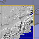
Using WCS data in a 2D GXY view samples.ogc.wcs.client.MainPanel
This sample demonstrates how to use an OGC Web Coverage Service (WCS) in a client application equipped with a 2D GXY view, using the Luciad WCS client API.
Using the client API, applications can create a "proxy" ILcdModel that transparently obtains coverage data from the WCS.
When a connection is made with a WCS service, the combo box in the upper right of the sample is populated with the list of coverages offered by this WCS. These coverages can be selected and visualized on the map.
Instructions
During startup, the sample will try to connect to one of two default OGC WCS services:
- a Luciad OGC WCS service sample running on localhost at port 8080 (http://localhost:8080/LuciadOGCServices/wcs). If the OGC
Web Services
Suite is available, this service can be started by running the
samples.ogc.server.Mainsample. - a public Luciad OGC WCS service (http://sampleservices.luciad.com/wcs).
Querying the list of available coverages: fill in a URL in the text field below the map and press the "Query WCS service" button. This will send a GetCapabilities request to the service and parse the list of available coverages. When successful, the coverages will be listed in the combo box in the upper right corner of the sample.
Retrieving and visualizing a coverage: select a coverage in the combo box in the upper right of the sample. Click the "Get coverage" button to send a GetCoverage request to the service and visualize the requested data on the map.
Using WFS data in a 2D GXY view samples.ogc.wfs.client.gxy.MainPanel
This sample demonstrates how to use an OGC Web Feature Service (WFS) in a client application equipped with a 2D GXY view, using the Luciad WFS client API.
Using the client API, applications can create a "proxy" ILcdModel that transparently obtains feature data from a WFS. This WFS proxy model can optionally be configured with an OGC Filter to be applied to the data and, as is done in the sample, a "maxfeatures" parameter to limit the number of features that are retrieved from the service.
When a connection is made with a WFS service, the combo box in the upper right of the sample is populated with the list of features types offered by this WFS. Selecting a feature types from the list retrieves and visualize the feature data on the map. You can also connect to other WFS services through the URL panel below the map.
Instructions
During startup, the sample will try to connect to one of two default OGC WFS services:
- a Luciad OGC WFS service sample running on localhost at port 8080 (http://localhost:8080/LuciadOGCServices/wfs). If the OGC
Web Services
Suite is available, this service can be started by running the
samples.ogc.server.Mainsample. - a public Luciad OGC WFS service (http://sampleservices.luciad.com/wfs).
To query the list of available feature types, fill in a server and press the "Query" button. This will send a GetCapabilities request to the service and parse the list of available features types. When successful, the feature types will be listed in the combo box in the upper right corner of the sample.
To visualize a feature type, just select it from the combo box. This will send a GetFeature request to the service for the selected feature type, and create a layer to visualize the retrieved feature data.
Using WFS data in a 2D / 3D Lightspeed view samples.ogc.wfs.client.lightspeed.MainPanel
This sample demonstrates how to use an OGC Web Feature Service (WFS) in a client application equipped with a 2D / 3D Lightspeed view, using the Luciad WFS client API.
Using the client API, applications can create a "proxy" ILcdModel that transparently obtains feature data from a WFS. This WFS proxy model can optionally be configured By default, this results in a map loaded with:
- the states and the rivers of the USA,
- the roads and a raster background of Washington DC,
- a blue polygon partially covering Canada.
When a connection is made with a WFS service, the combo box in the upper right of the sample is populated with the list of features types offered by this WFS. Selecting a feature types from the list retrieves and visualize the feature data on the map. You can also connect to other WFS services through the URL panel below the map.
Instructions
During startup, the sample will try to connect to one of two default OGC WFS services:
- a Luciad OGC WFS service sample running on localhost at port 8080 (http://localhost:8080/LuciadOGCServices/wfs). If the OGC
Web Services
Suite is available, this service can be started by running the
samples.ogc.server.Mainsample. - a public Luciad OGC WFS service (http://sampleservices.luciad.com/wfs).
To query the list of available feature types, fill in a server and press the "Query" button. This will send a GetCapabilities request to the service and parse the list of available features types. When successful, the feature types will be listed in the combo box in the upper right corner of the sample.
To visualize a feature type, just select it from the combo box. This will send a GetFeature request to the service for the selected feature type, and create a layer to visualize the retrieved feature data.

Using WMS data in a 2D GXY view samples.wms.client.gxy.MainPanel
This sample demonstrates how map data from an OGC Web Map Service (WMS) can be retrieved and visualized in a GXY (2D) view.
Using the client API, applications can create a "proxy" ILcdModel that transparently obtains map data from the WMS.
When a connection is made with a WMS service, the layer list in the upper right of the sample is populated with the list of layers offered by this WMS. These layers can be selected and visualized on the map.
You can switch between a tiled and a non-tiled painting strategy. Tiled painting typically offers better performance while non-tiled painting allows pixel-perfect results in a 2D view.
The sample also demonstrates the use of WMS feature info requests. If the WMS advertises GetFeatureInfo support, you can click on the map. This requests additional feature information for that location from the service. If feature information is available, it will be painted as an overlay label on the map at the clicked location.
The sample demonstrates making use of multi-dimensional data when selecting WMS layers for which the WMS server advertises them.
The check box "Auto-update WMS" is enabled by default, which means that the sample will check at each pan/zoom action whether the capabilities at the server have been updated. Any changes in the available layers are applied automatically; if there are any new layers defined at the server, they will be added. Layers that are not available anymore at the server will be removed automatically.
Instructions
During startup, the sample will try to connect to one of two default OGC WMS services:
- a Luciad OGC WMS service sample running on localhost at port 8080 (http://localhost:8080/LuciadOGCServices/wms). If the OGC
Web Services
Suite is available, this service can be started by running the
samples.ogc.server.Mainsample. - a public Luciad OGC WMS service (http://sampleservices.luciad.com/wms).
WMS layer selection: the list in the upper right of the samples shows the available WMS layers. Selecting and deselecting layers triggers a map refresh, taking into account the current WMS layer selection.
Map interaction: the toolbar offers a set of actions to navigate on and interact with the map. This includes the ability to pan and zoom, to measure distances and to switch the projection. When the selection projection does not match the available projects in the WMS service, the data is automatically reprojected, fully transparent for the user.
Painting settings: disable the tiled checkbox in the panel. The update latency will increase but the results are now pixel-perfect when the view is using a 2D reference that is supported by the WMS server.
Feature info: click on the crosshair button in the toolbar to activate the feature info controller. Clicking on the cities or rivers of the USA or on the streets of Washington DC shows a label with the feature information next to the clicked point, if available.
Enable the check box "Auto-update WMS" to let the application check for new/removed WMS layers at each pan or zoom action. When used with the sample Luciad WMS service, one can add data in the samples/resources/Data/dynamic folder to try this feature. The following data formats are supported: SHP, MIF, CADRG, DMED, DEM, GeoTIFF, raster (.rst), ETOPO and a custom format (.txt). This folder is monitored each 10 seconds. When new data is found or when data is removed, the advertised layers in the WMS capabilities are automatically updated, and the client sample will automatically pick up the changes. Newly added data should therefore soon become visible at the client, after a pan or zoom action.
Using WMS data in a 2D / 3D Lightspeed view samples.wms.client.lightspeed.MainPanel
This sample demonstrates how map data from an OGC Web Map Service (WMS) can be retrieved and visualized in a Lightspeed view.
Using the client API, applications can create a "proxy" ILcdModel that transparently obtains map data from the WMS.
When a connection is made with a WMS service, the layer list in the upper right of the sample is populated with the list of layers offered by this WMS. These layers can be selected and visualized on the map.
You can switch between a tiled and a non-tiled painting strategy. Tiled painting typically offers better performance while non-tiled painting allows pixel-perfect results in a 2D view.
The sample also demonstrates the use of WMS feature info requests. If the WMS advertises GetFeatureInfo support, you can click on the map. This requests additional feature information for that location from the service. If feature information is available, it will be painted as an overlay label on the map at the clicked location.
The sample demonstrates making use of multi-dimensional data when selecting WMS layers for which the WMS server advertises them.
Instructions
During startup, the sample will try to connect to one of two default OGC WMS services:
- a Luciad OGC WMS service sample running on localhost at port 8080 (http://localhost:8080/LuciadOGCServices/wms). If the OGC
Web Services
Suite is available, this service can be started by running the
samples.ogc.server.Mainsample. - a public Luciad OGC WMS service (http://sampleservices.luciad.com/wms).
WMS layer selection: the list in the upper right of the samples shows the available WMS layers. Selecting and deselecting layers triggers a map refresh, taking into account the current WMS layer selection.
Map interaction: the toolbar offers a set of actions to navigate on and interact with the map. This includes the ability to pan and zoom, to measure distances and to switch the projection. When the selection projection does not match the available projects in the WMS service, the data is automatically reprojected, fully transparent for the user.
Painting settings: disable the tiled checkbox in the panel. The update latency will increase but the results are now pixel-perfect when the view is using a 2D reference that is supported by the WMS server.
Feature info: click on the crosshair button in the toolbar to activate the feature info controller. Clicking on the cities or rivers of the USA or on the streets of Washington DC shows a label with the feature information next to the clicked point, if available.
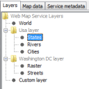
WMS Server Configuration Editor samples.wms.server.config.editor.MainPanel
This sample is a configuration editor for a Luciad Web Map Server.
Instructions
OGC services samples.ogc.server.Main
This sample starts the OGC web services sample on localhost port 8080, giving access to an OGC
Web Map Service (WMS), a Web Feature Service (WFS), and a Web Coverage Service (WCS).
LuciadFusion also adds a Web Catalogue Service (CSW) to this sample.
Instructions
The services can be accessed through a set of client samples delivered with LuciadLightspeed, or through the service's administrative page available at the following URL: http://localhost:8080/LuciadOGCServices This administrative page is built using HTML / JavaScript and is delivered with the services sample. It provides a graphical front-end to the OGC services and gives access to their capabilities.
You can run one of the client samples delivered with LuciadLightspeed to connect with the OGC services:
- Using WMS data in a 2D GXY view
- Using WMS data in a 2D / 3D Lightspeed view
- Using WFS data in a 2D GXY view
- Using WFS data in a 2D / 3D Lightspeed view
- Using WCS data in a 2D GXY view
Fusion LTS service samples.fusion.server.Main
This sample starts the Fusion LTS service sample on localhost port 8082, giving access to a
LuciadFusion Tile Store (LTS).
Instructions
The service can be accessed through a client sample delivered with LuciadFusion, or through the service's administrative page available at the following URL: http://localhost:8082/LuciadFusion This administrative page is built using HTML / JavaScript and is delivered with the service sample. It provides a graphical front-end to the Fusion LTS service and gives access to its capabilities.
You can run one of the client samples delivered with LuciadFusion to connect with the LTS service:
- GXY: Decoding multiple format data (samples.gxy.decoder.MainPanel)
- Lightspeed: Decoding multiple format data (samples.lightspeed.decoder.MainPanel)
Adding custom profiles to differentiate between deployment environments for the Fusion Platform samples.fusion.platform.profiles.CustomProfilesFusionPlatformApplication
This sample demonstrates how to create your own Spring profiles. This is a useful feature that can be used to have different configurations in different environments without changing anything in your application.
For the sake of simplicity, the sample application activates the custom staging profile programmatically. The preferred way of setting the active profile is to use program arguments, vm parameters or JNDI attributes. See the deployment guide for more information about Spring profiles.
Using Spring Security to perform database authentication samples.fusion.platform.security.authentication.CustomAuthenticationFusionPlatformApplication
This sample demonstrates how to create your own authentication logic. This implementation intends to replace the default built-in LuciadFusion Platform security authentication logic. This is useful in scenarios where users intend to implement their own user authentication logic. For the sake of simplicity, this sample uses user authentication via a database, but the concept can be extended to implement more complex authentication logic.
Using Spring Security to perform user authorization in order to restrict access to HTTP resources samples.fusion.platform.security.http.CustomHttpSecurityFusionPlatformApplication
This sample demonstrates how to create your own authorization logic. This implementation intends to replace the default built-in LuciadFusion Platform HTTP security configuration. This is useful in scenarios where users intend to implement their own security and authorization logic.
Extending LuciadFusion Platform with a custom Spring endpoint samples.fusion.platform.service.CustomServiceFusionPlatformApplication
Example Fusion application to create an extra Spring endpoint. In this case a simple "Hello World" service, that exposes the "/hello" and "/hello/{name}" endpoints.

Adding a custom service type to LuciadFusion (SHP Quiz) samples.fusion.platform.shpquiz.FusionServerSampleShpQuiz
Custom service type example.
This sample shows how to add a custom service type that can be used within LuciadFusion Studio. A SHP Quiz service type is added that creates quizzes from SHP files published in the services of this type.
Advanced GIS Engine

GXY: Constructive Geometry samples.geometry.constructive.gxy.MainPanel
This sample allows performing convex hull operation and constructive geometry operations on interactively created shapes.
Instructions
To apply convex hull and constructive geometry operations to a shape you created and edited:
- Click one of the new shape buttons in the toolbar and click on the map to create a new shape.
- Edit a shape in the user layer by dragging one of its points or segments
- Calculate the convex hull of a shape by selecting one shape, right clicking and choosing Convex Hull from the menu
- Calculate a boolean operation of two shapes by selecting two shapes, right clicking and choosing Intersection, Union, Difference, Inverted Difference or Symmetric Difference from the menu
Lightspeed: Constructive Geometry samples.geometry.constructive.lightspeed.MainPanel
This sample allows performing convex hull operation and constructive geometry operations on interactively created shapes.
Instructions
To apply convex hull and constructive geometry operations to a shape you created and edited:
- Click one of the new shape buttons in the toolbar and click on the map to create a new shape.
- Edit a shape in the user layer by dragging one of its points or segments
- Calculate the convex hull of a shape by selecting one shape, right clicking and choosing Convex Hull from the menu
- Calculate a boolean operation of two shapes by selecting two shapes, right clicking and choosing Intersection, Union, Difference, Inverted Difference or Symmetric Difference from the menu
Ellipsoidal Geometry samples.geometry.topology.ellipsoidal.MainPanel
This applet demonstrates several topological relations provided by the rigorous geometry package. The relations can be checked between US states and geodetic flight trajectories. It's possible to select an object. All other objects are then color-coded according to their relationship with the selected object. Not all possible relations supported by the package are shown and if multiple relations hold true only one is shown, otherwise too much different colors would be needed.
Instructions
States and flight trajectories are shown in gray by default. Use the selection tool to select a state or a flight trajectory. All other objects that interact with the selected object in some way are then drawn in another color. The color codes are:
- White: Disjoint with selected object
- Green: Selected object
- Yellow: Crosses selected object
- Red: Touches selected object
- Blue: Contains or within selected object.
- Cyan: Intersects the selected object in any other way. This color is overridden by crosses, touches, contains or within if one of those is true.

Interactive samples.geometry.topology.interactive.MainPanel
This applet allows creating shapes using toolbar buttons and editing them. Selecting two shapes displays their topology relations.
Instructions
To analyze the topology relations between two shapes you created and edited:
- Click one of the new shape buttons in the toolbar and click on the map to create a new shape.
- Edit a shape in the user layer by dragging one of its points or segments
- Calculate the topology relations of two shapes by selecting these two shapes
Advanced Raster Services
Panorama converter samples.panorama.converter.PanoramaConverter
This is a command-line sample. Click More info for run instructions.
This command-line tool demonstrates how to convert any data format that contains valid Panoramic image data into the Luciad Panorama Format. The Luciad Panorama Format is optimized for serving the Panoramic image data with LuciadFusion and visualizing with LuciadRIA. Refer to the Panoramic image section of the documentation for more information.
Run the sample using the shell script in the samples folder:
panorama.converter.bat -i=<inputFile> -o=<outputFile>
Panorama Viewer samples.panorama.viewer.MainPanel
This sample can visualize panorama locations on the map, display the raw images and process them into a Luciad Panorama.
Instructions
-
Load a panorama dataset.
The panorama positions are displayed on the map as points. -
Select a panorama on the map.
The image(s) of the panorama are displayed on the left. Use the combobox at the bottom to select a specific image. -
Process the selected panorama into a Luciad Panorama.
The resulting cubemap images are displayed on the right.
This sample can be used as a debugging tool when implementing a custom panorama format.
The Luciad Panorama is not stored, use the Panorama Converter sample or LuciadFusion to fully process panoramas.
Refer to the Panoramic images section of the documentation.
Database Connectors
DB2 Spatial Encoder Sample samples.encoder.db2.spatial.Main
This is a command-line sample. Click More info for run instructions.
This application demonstrates how to encode spatial data to an DB2 Spatial database, using a TLcdDB2SpatialModelEncoder.
Run the sample using the shell script in the samples folder:
encoder.db2.spatial.bat source_file destination_db2_file
The connection to the database can be specified by means of a properties
file, in this case Data/Db2/states.db2.
To convert a file, make sure the URL in Data/Db2/states.db2 points to your
DB2 Spatial database and convert for example Data/Shp/Usa/states.shp into it.
Informix Geodetic Encoder Sample samples.encoder.informix.geodetic.Main
This is a command-line sample. Click More info for run instructions.
This application demonstrates how to encode geodetic data to an Informix Geodetic database, using a TLcdInformixGeodeticModelEncoder.
Run the sample using the shell script in the samples folder:
encoder.informix.geodetic.bat source_file destination_ifx_file
The connection to the database can be specified by means of a properties
file, in this case Data/Informix/states.ifx.
Make sure the URL in Data/Informix/states.ifx points to your
Informix Geodetic database. You can then convert Data/Shp/Usa/states.shp
to Data/Informix/states.ifx
Informix Spatial Encoder Sample samples.encoder.informix.spatial.Main
This is a command-line sample. Click More info for run instructions.
This application demonstrates how to encode spatial data to an Informix Spatial database, using a TLcdInformixSpatialModelEncoder.
Run the sample using the shell script in the samples folder:
encoder.informix.spatial.bat source_file destination_isd_file
The connection to the database can be specified by means of a properties
file, in this case Data/Informix/states.isd.
Make sure the URL in Data/Informix/states.isd points to your
Informix Spatial database. You can then convert
Data/Shp/Usa/states.shp to Data/Informix/states.isd
Microsoft SQL Encoder Sample samples.encoder.mssql.Main
This is a command-line sample. Click More info for run instructions.
This application demonstrates how to encode spatial data to a Microsoft SQL database, using a TLcdMSSQLModelEncoder.
Run the sample using the shell script in the samples folder:
encoder.mssql.bat source_file destination_mss_file
The connection to the database can be specified by means of a properties
file, in this case Data/MSSQL/world.mss.
Make sure the URL in Data/MSSQL/world.mss points to
your Microsoft SQL database. You can then convert
Data/Shp/world/world.shp to Data/MSSQL/world.mss.
Oracle Spatial Object-Relational Encoder Sample samples.encoder.oracle.spatial.Main
This is a command-line sample. Click More info for run instructions.
This application demonstrates how to encode spatial data to an Oracle Spatial Object-Relational database, using a TLcdOracleSpatialModelEncoder.
Run the sample using the shell script in the samples folder:
encoder.oracle.spatial.bat source_file destination_ora_file
The connection to the database can be specified by means of a properties
file, in this case Data/Oracle/states.ora .
Make sure the URL in Data/Oracle/states.ora points to your
Oracle Spatial database. You can then convert
Data/Shp/Usa/states.shp to Data/Oracle/states.ora.
PostgreSQL PostGIS Encoder Sample samples.encoder.postgresql.Main
This is a command-line sample. Click More info for run instructions.
This application demonstrates how to encode spatial data to a PostgreSQL PostGIS database, using a TLcdPostGISModelEncoder.
Run the sample using the shell script in the samples folder:
encoder.postgresql.bat source_file destination_pgs_file
The connection to the database can be specified by means of a properties
file, in this case Data/Postgresql/states.pgs .
Make sure the URL in Data/Postgresql/states.pgs points to
your PostgreSQL PostGIS database. You can then convert
Data/Shp/Usa/states.shp to Data/Postgresql/states.pgs.
SAP Hana sample samples.hana.lightspeed.MainPanel
- STORMS: shapes representing windspeeds at a certain time - based on the Sandy hurricane
- CUSTOMERS: points representing insurance company policy holders - semi-random
Instructions
- See how many policy holders are affected, per US state and county
- See a heat map of the customers
- See individual customers as icons, and filter on them
Graph and Routing Engine
Network analysis of GDF data samples.decoder.gdf.network.MainPanel
This sample shows how to integrate network functionality in GDF applications. GDF datasets can be read into the sample. During loading, the sample will convert the GDF data into a road network and preprocess the network. The network toolbar provides all functionality to compute shortest routes and traces on the road network. The info button shows details about all routes/traces which are computed.
Instructions
First select a GDF file using the 'Open' button in the toolbar. After the data has been loaded, shortest routes can be computed and displayed. To compute a route:
- Press the "Select start node" button and choose a start node on the map (only the begin and end point of roads (polylines) are selectable).
- Press the "Select end node" button and choose a end node on the map (only the begin and end point of roads (polylines) are selectable).
- Press the "Calculate the shortest route" button to compute and visualize the shortest route.
Network analysis samples.network.basic.MainPanel
This sample demonstrates how to use the LuciadLightspeed Graph & Routing Engine component. It contains a sample graph, representing a small road network, consisting of a set of nodes (junctions) and edges (roads) connecting the nodes. Some of the roads are directed (indicated by a black arrow), some turns are forbidden (indicated by a red corner). Each road has an associated maximum speed, indicated by its thickness.
The length of a route is defined by an ILcdEdgeValueFunction, which associates a value with each edge in the graph. This value can be based on a simple cartesian distance function, a function combining distance and maximum speed into a time-cost function, or other, user-defined functions.
You can display the complete sequence of edges and the total distance of a route via the 'Show routing information' button.
The sample also illustrates how to associates values with nodes, e.g. to incorporate the time to wait for a traffic light on a junction.
Heuristic distance functions, providing estimate distances between two nodes, can accelerate the routing process. They are not required for the routing algorithm to work, but, if one is used, the calculated distances should always be an underestimate of the real remaining distance, otherwise a correct result is not guaranteed.
The cost function and heuristic distance function to be used can be configured via the 'Network configuration' button.
Besides routing, tracing can also be performed, calculating all nodes that are reachable within a given distance.
Finally, the sample shows how to partition a graph and perform routing in partitioned graphs. A partition is calculated for the sample graph, and is visualized by the colors of the nodes. Partitioning can reduce the processor and memory usage significantly when routing.
Note that the size of this sample graph is too small to show the effect of heuristic distance functions and partitioning on routing performance.
Instructions
Routes can be calculated by first selecting a start node and an end node, using the start/end node selection controller. Once start node and end node are selected, the route can be computed and visualized by pressing the 'Calculate the shortest route' button. Optionally, a start and/or end edge can also be selected, but they are only relevant when turn restrictions are activated. The start and end edge should always be connected to the start and end node, respectively.
Cross country network analysis samples.network.crosscountry.MainPanel
This sample demonstrates how to perform cross country route planning with LuciadLightspeed. The sample shows a map with height data. The "Compute route" controller allows to select two points. After the second point has been selected, a route between the two selected points will be computed and shown.
The right panel allows to experiment with different distance functions, which will result in different solutions.
Heuristic distance functions, providing estimate distances between two nodes, can accelerate the routing process. They are not required for the routing algorithm to work, but, if one is used, the calculated distances should always be an underestimate of the real remaining distance, otherwise a correct result is not guaranteed. The right panel allows to enable or disable a simple distance function.
Note that, since the algorithm uses a raster approximation, the computed solution will be an approximation of the actual shortest route.
Instructions
To compute a route, first enable the "Compute route" controller by pressing the "Compute route" button. After the controller has been enabled, select a start and end point on the map. After the second point has been selected, a route between the two selected points will be computed and shown.
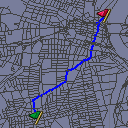
Numeric network viewer samples.network.numeric.MainPanel
This sample demonstrates how to analyze very large networks with LuciadLightspeed, using numeric graphs. The sample has an Open button which allows to load a numeric graph that was created with the network preprocessor sample. By default, the sample will load the USA roads dataset included in the release.
After the graph has been loaded, routes can be calculated by first selecting a start and end node via the start/end node selection controller, and then pressing the routing button. Only begin and end points of roads (polylines) can be selected as start/end node. Optionally, a start edge can also be selected to indicate from which direction the beginning of the route will be entered, and an end edge to indicate in which direction the route will be left. The start and end edge should always be connected to the start and end node, respectively. They are only relevant however when the graph contains turn restrictions.
The 'Destroy edge' button allows to mark edges as deleted. The application will take these changes into account during succeeding shortest route computations.
Note the sample has a scale range set on the layers, as the default sample dataset is too large to display at once on the map. Zoom in on the map to make the data visible.
Instructions
First preprocess a SHP file using the samples.network.numeric.preprocessor sample. The generated Network configuration properties file can be loaded using the 'Open file' button. After the data has been loaded, shortest routes can be computed and displayed. To compute a route:
- Press the "Select start node" button and choose a start node on the map.
- Press the "Select end node" button and choose a end node on the map.
- Press the "Calculate the shortest route" button to compute and visualize the shortest route.
Numeric network preprocessor samples.network.numeric.preprocessor.Main
This is a command-line sample. Click More info for run instructions.
This command-line tool demonstrates how to convert SHP data to a numeric graph.
Run the sample using the shell script in the samples folder:
network.numeric.preprocessor.bat source_directory destination_file
This sample is a command-line sample.
It requires two arguments: one specifying the data source dir and one specifying the
numeric graph destination file.
A sample dataset is provided in resources/Data/Shp/Usa/roads/.
Instructions
See the documentation of Preprocessor.java for more information on how the input data should be organized.
The properties file that is created by the preprocessor can be opened with the numeric network viewer sample.
Real-time Engine
GXY: Cluster labeling samples.realtime.gxy.clusterLabeling.MainPanel
This sample shows how to interactively declutter clusters of objects using offset icons, the continuous labeling algorithm and an animation labeling algorithm. A discrete labeling algorithm declutters the labels statically. When the mouse hovers over a cluster, the icons are first animated by an animation labeling algorithm, and then decluttered using the continuous labeling algorithm.
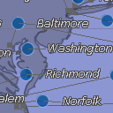
GXY: Offset icons samples.realtime.gxy.offsetIcon.MainPanel
This sample demonstrates how to combine offset label placement and continuous label decluttering. It also shows how to customize the labeling algorithm by
- adjusting the desired label locations: the desired label location of the icon labels is the upper right of the city. The desired location of the text labels is on the right of the icon labels.
- configuring the master-slave dependency: when the icon label is moved, the text label moves along.
- dropping overlapping labels.
- never dropping a text-label without first dropping the offset icon to which it belongs.
Instructions
Lightspeed: Cluster labeling samples.realtime.lightspeed.clusterLabeling.MainPanel
This sample shows how to interactively declutter clusters of objects using offset icons, the continuous labeling algorithm and an animation labeling algorithm. A discrete labeling algorithm declutters the labels statically. When the mouse hovers over a cluster, the icons are first animated by an animation labeling algorithm, and then decluttered using the continuous labeling algorithm.
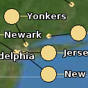
Lightspeed: Offset icons samples.realtime.lightspeed.offsetIcon.MainPanel
This sample demonstrates how to combine offset label placement and continuous label decluttering. It also shows how to customize the labeling algorithm by
- adjusting the desired label locations: the desired label location of the icon labels is the upper right of the city. The desired location of the text labels is on the right of the icon labels.
- configuring the master-slave dependency: when the icon label is moved, the text label moves along. The text label can be moved independently from the icon label.
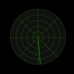
Lightspeed: Radar sweeps samples.realtime.lightspeed.radarvideo.RadarVideoSample
This sample demonstrates how to connect to and visualize a custom radar feed. This sample uses the following classes:
TLcdRadar: the domain object into which you decode your radar video dataTLspRadarVideoLayerBuilder: the layer builder for showing the radar video data in a Lightspeed view
Instructions
Configure the styling of the radar using the controls in the bottom right panel. You can change the following properties of the styling:
- Colors: change the color of the background, sweep and blips.
- Enable or disable the sweep and grid lines.
Switch to different 2D projections to see how the radar display is warped. Switch to 3D to see how the radar feed is draped on the terrain.
Terrain Analysis Engine
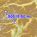
GXY: Measuring distance over terrain samples.tea.gxy.distance.MainPanel
This sample demonstrates the terrain distance controller.
The terrain distance controller measures distance between points taking into account the terrain elevation in between. As such this will be an approximation of the distance to travel over land from start to end point.
The distance is influenced by the path taken between the points which can be either geodetic (shortest path on the ellipsoid) or of constant azimuth. Note that distance following a constant azimuth path may be smaller than when following a geodetic path, due to the terrain underneath.
Instructions
Activate the terrain ruler in the toolbar and click a few times on the DTED data. A path is created and the distance along that path is shown computed. Adjust the measure mode settings to use a different distance calculation. Notice how the distance is bigger if “over terrain” is enabled. The parts of the measurement that are out of terrain bounds are shown as “Unknown”.
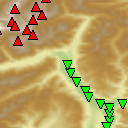
GXY: Finding the extreme points inside a shape samples.tea.gxy.extremepoint.MainPanel
This sample demonstrates how to find extreme points inside a shape.
The sample allows you to find minimum and maximum points inside a selected area. A minimum/maximum point is defined to be the lowest or highest point in the surrounding area. This area is defined by a configurable separation distance. You can set this value to infinity which means the separation height requirement applies to the entire map, not just the surrounding area.
To ensure that the peaks are more or less distinct, a separation height is needed. This height defines the minimum height difference which has to be bridged between two peaks. You can set this value to infinity which means no other peak can be found within the separation distance.
Instructions
Edit the selected polygon, adjust the extreme point settings and click the 'Compute' button. The found minimum (green) and maximum (red) points are added to the map and are shown inside the polygon.
GXY: Hypsometric computations samples.tea.gxy.hypsometry.MainPanel
This sample demonstrates how to visualize hypsometric computations on elevation data in a Lightspeed view. The computations can be applied to either the view's terrain or a specific elevation model.
Instructions
The application generates all hypsometric calculations in advance, and puts them in separate layers. You can view the different hypsometric functions separately by toggling the visibility of their respective layers. The following functions are shown:
- Ridges and valleys: Blue indicates ridges, red indicates valleys.
- Shading: Applies a shading function based on the slope and orientation. Hill sides facing away from the reference direction are dark, sides facing along the reference direction are bright.
- Orientation: Computes the angle of steepest descent. Hills facing along the reference direction are blue, the opposite sides are red.
- Slope: Determines the angle between the normal of a point and the input angles. Flat areas are green, hill sides are colored according to their steepness (yellow – red – black).
- Azimuth: Determines the azimuth of a point.
The panel in the upper right corner displays information about the hypsometric functions, relative to the position of the mouse.
GXY: Line-of-sight samples.tea.gxy.los.MainPanel
This sample demonstrates how to produce line-of-sight computations, between two points and between a point and its environment.
The map shows DTED terrain data and points defined in a geodetic reference (black with white border) and in a grid reference (white with black border).
Instructions
For point-to-point computations:
- open the input dialog and select two points on the map
- enter the heights above terrain for both points
- select the layer the result should be put in
- enter the distance (in meters) between the intermediate points
- press the compute button
For line-of-sight coverage computations:
- open the input dialog and select a point on the map
- enter the radius and angles and the height above ground
- enter the steps for the intermediate points or choose to have them computed automatically (in advanced mode)
- enter the visibility parameters
- choose the computation algorithm
- set how the result should be interpreted. Minimum typically results in more red pixels, maximum in more green pixels. In mountainous areas the difference between minimum and maximum is typically larger than in flat valleys.
- select the layer the results should be put in
- optionally, fill in or compute the density of the sampling (in advanced mode)
- press the compute button
GXY: Directional Viewshed samples.tea.gxy.viewshed.directional.MainPanel
This sample demonstrates how to generate directional viewsheds for terrain and a shape model.
Instructions
To calculate shadows for the sample terrain and city:
- Select the position of the sun by inputting its coordinates or dragging around the sun icon. For example, (0.0,0.0) means that the sun will be at position (0.0,0.0) at infinite height.
- Enter a sampling height offset. For example, 1.0m means that the visibility of a lon-lat coordinate will be determined one meter above ground.
- Enter a terrain step size. For example, 100m means that terrain will be sampled once every 100 meters. Note that smaller step sizes will require more calculations.
- Hit the update button.
The sample creates a new composite viewshed based on the terrain and the city. It does so by extruding the given polygons to make them 3D. It also places the resulting extruded shapes above terrain. The sun is used as a direction: Conceptually the sun is at infinite height.
To visualize the viewshed it is wrapped in a multilevel raster. Visible (i.e. non-shadowed) portions of the terrain are transparent, while non-visible (i.e. shadowed) portions are gray. The raster creates tiles by sampling the composite viewshed at a height that is a combination of the height of the terrain plus the sampling height offset.
GXY: Positional Viewshed samples.tea.gxy.viewshed.positional.MainPanel
This sample demonstrates how to generate positional viewsheds for terrain and a shape model.
Instructions
To calculate visibility for the sample terrain and city:
- Select the position of the observer by inputting its coordinates or dragging around the green observer icon.
- Enter an eye height offset. For example, 2.0m means that the observer is 2 meters above ground.
- Enter a sampling height offset. For example, 1.0m means that the visibility of a lon-lat coordinate will be determined one meter above ground.
- Enter a terrain step size. For example, 100m means that terrain will be sampled once every 100 meters. Note that smaller step sizes will require more calculations.
- Hit the update button.
The sample creates a new composite viewshed based on the terrain and the city. It does so by extruding the given polygons to make them 3D. It also places the resulting extruded shapes above terrain. The observer is used as a position. Its height is given by the underlying terrain, plus the eye height offset.
To visualize the viewshed it is wrapped in a multilevel raster. Visible portions of the terrain are transparent, while non-visible portions are gray. The raster creates tiles by sampling the composite viewshed at a height that is a combination of the height of the terrain plus the sampling height offset.
GXY: Computing the visibility of a polyline or a polygon from another shape samples.tea.gxy.visibility.MainPanel
The sample allows you to compute the visibility from a shape to a polyline or a polygon. You can do so by specifying the shapes using the drop-downs.
Instructions
Edit the shapes and configure the desired visibility computation with the drop-downs. The visibility will be computed and added to the map.
- The result of a 'to polyline' visibility computation is drawn on top of the polyline as green and red lines indicating which parts of the shape are visible and which are not.
- The result of a 'to polygon' visibility computation is drawn as a raster inside the bounds of the polygon. Areas with green raster pixels are visible, areas with red pixels are invisible.
- Visibility is recomputed when you edit one of the two shapes involved in the current visibility setting. If the previous computation has not yet completed, the intermediate result is shown.
Lightspeed: Contours samples.tea.lightspeed.contour.MainPanel
This sample demonstrates the contour functionality of the Terrain Analysis Engine Component.
Instructions
Select a type of contour. Two different contour types are available:
- polygon contours
- polyline contours. Zoom in to see labels showing the height of the contours.
Lightspeed: Measuring distance over terrain samples.tea.lightspeed.distance.MainPanel
This sample demonstrates the terrain distance controller.
The terrain distance controller measures distance between points taking into account the terrain elevation in between. As such this will be an approximation of the distance to travel over land from start to end point.
The distance is influenced by the path taken between the points which can be either geodetic (shortest path on the ellipsoid) or of constant azimuth. Note that distance following a constant azimuth path may be smaller than when following a geodetic path, due to the terrain underneath.
Instructions
Activate the terrain ruler and click a few times on the DTED data. A path is created and the distance along that path is shown computed. Adjust the measure mode settings to use a different distance calculation. Notice how the distance is bigger if “over terrain” is enabled. The parts of the measurement that are out of terrain bounds are shown as “Unknown”.
Lightspeed: Finding the extreme points inside a shape samples.tea.lightspeed.extremepoint.MainPanel
This sample demonstrates how to find extreme points inside a shape.
The sample allows you to find minimum and maximum points inside a selected area. A minimum/maximum point is defined to be the lowest or highest point in the surrounding area. This area is defined by a configurable separation distance. You can set this value to infinity which means the separation height requirement applies to the entire map, not just the surrounding area.
To ensure that the peaks are more or less distinct, a separation height is needed. This height defines the minimum height difference which has to be bridged between two peaks. You can set this value to infinity which means no other peak can be found within the separation distance.
Instructions
Edit the selected polygon, adjust the extreme point settings and click the 'Compute' button. The found minimum (green) and maximum (red) points are added to the map and are shown inside the polygon.
Change the DTED level to control the resolution of the height data for the search algorithm.
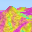
Lightspeed: Hypsometric computations samples.tea.lightspeed.hypsometry.MainPanel
This sample demonstrates how to visualize hypsometric computations on elevation data in a Lightspeed view. The computations can be applied to either the view's terrain or a specific elevation model.
Instructions
Explore the various hypsometric functions and their input parameters (if applicable):
- Ridges and valleys: Blue indicates ridges, red indicates valleys.
- Shading: Applies a shading function based on the slope and orientation. Hill sides facing away from the reference direction are dark, sides facing along the reference direction are bright.
- Orientation: Computes the angle of steepest descent, relative to the input angles. Hills facing along the reference direction are blue, the opposite sides are red.
- Slope: Determines the angle between the normal of a point and the input angles. Flat areas are green, hill sides are colored according to their steepness (yellow – red – black). The values reflect the angle between a hill side and the reference direction, so at low vertical angles only steep hills facing towards the horizontal reference direction are highlighted.
- Azimuth: Determines the azimuth of a point, as determined by the normal, relative to the input parameters. Hill sides are colored based on their angle relative to the horizontal angle control.
Open some additional elevation data (for example Data/Dted/Alps/dmed) and select the layer in the combo box in the "Hypsometry Data" panel. The hypsometric computations are now only applied to the selected layer instead.
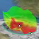
Lightspeed: Line Of Sight samples.tea.lightspeed.los.MainPanel
This sample demonstrates how to set up Line-of-Sight (LOS) calculations in a Lightspeed view. The sample allows the user to edit an arcband that is used as input for LOS calculation.
The input shape is edited using the default shape editor. The resulting Line-of-Sight shape is visualized as a three-dimensional sheet using a TLspLOSCoveragePainter.
Instructions
To edit the LOS calculation, first select the LOS input shape by clicking on it.
You can change the shape as follows:
- move around the center point by dragging around the input shape
- increase or decrease the radius of the LOS calculation by dragging the outer radius handles. The radius of the LOS input shape is limited in its size for this sample.
- limit the arcband range of the LOS calculation by dragging the outer radius handles
Use the sliders in the parameters panel on the right to modify:
- The angular step size, in degrees
- The radial step size, in metres
- The relative increase of subsequent radial step sizes, in %. If not zero, the radial steps increase outward from the center of the LOS coverage. This is for example useful to reduce the performance impact of large radius/small (initial) step size combinations. The effect is more easily noticeable when the radius is large and a non-gradient color map is used.
- The altitude of the center point, in metres above ground.
- The minimal vertical angle for the cone of silence, in degrees.
- The maximal vertical angle for the cone of silence, in degrees.
The style panel in the upper right side of the screen controls the following parameters:
- The colors at certain altitudes
- The opacity of the LOS colors
- Toggle draping for the LOS visualization. The calculation is projected onto the terrain when on.
All changes are applied immediately.
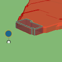
Lightspeed: Positional Viewshed samples.tea.lightspeed.viewshed.positional.MainPanel
This sample demonstrates how to generate positional viewsheds for terrain and a shape model.
Instructions
To calculate visibility for the sample terrain and city:
- Select the position of the observer by inputting its coordinates or dragging around the observer icon.
- Enter an eye height offset. (Example: 2.0m means that the observer is 2 meters above ground.)
- Enter a viewshed step size. (Example: 2.0m means that the visibility will be sampled once every 2.0 meters near the observer. Larger step sizes are used farther away.)
- Enter a terrain step size. (Example: 100m means that terrain will be sampled once every 100 meters.)
- Hit the update button.
After some seconds, a viewshed is shown, indicating the hidden areas for the observer. It does not perfectly fit the buildings because of the sampling resolution.
The visibility result (in the form of a viewshed) produces a scalar field. The viewshed is visualized using the marching cubes algorithm. This algorithm extracts a polygonal mesh from a three-dimensional scalar field. The mesh represents the volumes that are invisible to the observer. The algorithm samples the scalar field at certain locations. The UI allows you to specify the resolution of this sampling with the "Viewshed step size"-setting.
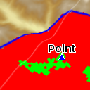
Lightspeed: Computing the visibility of a polyline or a shape from another shape samples.tea.lightspeed.visibility.MainPanel
The sample allows you to compute the visibility from a shape to a polyline or a polygon. You can do so by specifying the shapes using the drop-downs.
Instructions
Edit the shapes and configure the desired visibility computation with the drop-downs. The visibility will be computed and added to the map.
- The result of a 'to polyline' visibility computation is drawn on top of the polyline as green and red lines indicating which parts of the shape are visible and which are not.
- The result of a 'to polygon' visibility computation is drawn as a raster inside the bounds of the polygon. Areas with green raster pixels are visible, areas with red pixels are invisible.
- Visibility is recomputed when you edit one of the two shapes involved in the current visibility setting. If the previous computation has not yet completed, the intermediate result is shown.
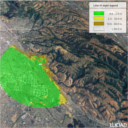
Adding a TEA (Terrain Elevation Analysis) custom service type to the LuciadFusion Platform samples.fusion.platform.tea.FusionServerSampleTea
Example TEA web service application using a custom service type.
The API documentation is integrated within the service.
After creating a TEA service in LuciadFusion Studio the documentation is available at
http://localhost:8081/samples/fusion/tea/{serviceName}/apidoc/index.html.
Weather & Environment Standards
GXY: displaying NetCDF and GRIB data samples.decoder.netcdf.gxy.MainPanel
This application demonstrates how to decode and visualize NetCDF and GRIB data.
The bottom of the map displays the data values under the mouse location. For every type of data, the value of the topmost visible layer is displayed.
The top of the map displays a time slider for temporal data. If there is no visible layer with time data, the slider is not displayed.
The left of the map displays a drop box menu and a vertical slider to filter multi-dimensional NetCDF and GRIB data. The menu allows you to choose one dimension, for example depth or air pressure. If there is no visible multi-dimensional layer, the slider and the menu are not displayed.
Notice that "Zonal Current" and "u,v-component of wind @ Isobaric surface" layers are interpolated on the dimensions.
Instructions
The decoder supports equally-spaced rectilinear grids that follow the NetCDF Climate and Forecast conventions and GRIB data. You can open such a file by clicking the Open toolbar button or by dragging a file onto the map. Move the mouse around to see the relevant data values.
Lightspeed: displaying NetCDF and GRIB data samples.decoder.netcdf.lightspeed.MainPanel
This application demonstrates how to decode and visualize NetCDF and GRIB data.
The bottom of the map displays the data values under the mouse location. For every type of data, the value of the topmost visible layer is displayed.
The top of the map displays a time slider for temporal data. If there is no visible layer with time data, the slider is not displayed.
The left of the map displays a drop box menu and a vertical slider to filter multi-dimensional NetCDF or GRIB data. The menu allows you to choose one dimension, for example depth or air pressure. If there is no visible multi-dimensional layer, the slider and the menu are not displayed.
Notice that "Zonal Current" and "u,v-component of wind @ Isobaric surface" layers are interpolated on the dimensions.
Instructions
The decoder supports equally-spaced rectilinear grids that follow the NetCDF Climate and Forecast conventions and GRIB files. You can open such a file by clicking the Open toolbar button or by dragging a file onto the map. Move the mouse around to see the relevant data values.
Aviation Standards
GXY: displaying AIS objects samples.ais.gxy.MainPanel
This sample demonstrates creation and display of aeronautical data using the LuciadLightspeed Aviation Standards component. The sample sets up a GXY view and adds a few layers with Aeronautical Information System (AIS) data. Models containing AIS objects are created in the ModelFactory class. Layer creation is performed in the LayerFactory class.
The data is generated in a geodetic model reference. This illustrates the use of the AIS shape classes.
Instructions
- Start the sample
- Select any of the features (airspace, procedure, airport) to see its label.
- Double-click on one of the features to show a dialog box containing its properties.
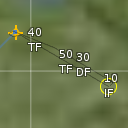
Lightspeed: display AIS objects samples.ais.lightspeed.MainPanel
This sample demonstrates creation and display of aeronautical data using the LuciadLightspeed Aviation Standards component. The sample sets up a Lightspeed view and adds a few layers with Aeronautical Information System (AIS) data. Models containing AIS objects are created in the ModelFactory class. Layer creation is performed in the LayerFactory class.
The data is generated in a geodetic model reference. This illustrates the use of the AIS shape classes.
Instructions
- Start the sample
- Select any of the features (airspace, procedure, airport) to see its label.
- Double-click on one of the features to show a dialog box containing its properties.
GXY: displaying AIXM data samples.decoder.aixm.gxy.MainPanel
This sample demonstrates how to load and display data in the AIXM 3.3, 4.0 and 4.5 format. The loading of the data relies on the use of the TLcdAIXMModelDecoder class in combination with a number of ILcdAIXMHandler implementation that each take care of one or more AIXM feature types (airspaces, routes, ...). The visualization is configured in the LayerFactory class.
Instructions
Press the open button in the toolbar to choose an AIXM snapshot or update file. You can select any of the loaded features to show a label, or you can double click on a feature to show the properties of the feature that were decoded from the AIXM file.
GXY: display AIXM 5.1 data samples.decoder.aixm51.gxy.MainPanel
This applet demonstrates how to create, load, store, and display AIXM data in a GXY view. The sample creates and displays an AIXM 5.1 designated point and airspace and loads some AIXM 5.1 data of the Chicago area. It also converts data from AIXM 4.5/3.3.
Instructions
If you want to use your own data, press the open button in the toolbar to choose an AIXM file. AIXM 5.1 files will be loaded directly, while airports, heliports and airspaces in AIXM4.5 and AIXM3.3 files will be converted on-the-fly to AIXM5.1 data.
Right click on an AIXM 5.1 feature on the map and choose 'View Properties' to show the data for that feature. The sample class AIXM51ElementFormatter is used by the dialog box to create more readable descriptions of the data. It also shows how to navigate through the domain model.
Select a layer and make it editable to enable editing of the AIXM 5.1 features. If you select a feature
and drag one of the handles, the underlying AIXM 5.1 data will be changed.
Click the save button to save the message in that layer to a file.
Lightspeed: display AIXM 5.1 data samples.decoder.aixm51.lightspeed.MainPanel
This applet demonstrates how to create, load, store, and display AIXM data in a Lightspeed view. The sample creates and displays an AIXM 5.1 designated point and airspace and loads some AIXM 5.1 data of the Chicago area.
Instructions
If you want to use your own data, press the open button in the toolbar to choose an AIXM file.
Right click on an AIXM 5.1 feature on the map and choose 'View properties' to show the data for that feature. The sample class AIXM51ElementFormatter is used by the dialog box to create more readable descriptions of the data. It also shows how to navigate through the domain model.
Select a layer and make it editable to enable editing of the AIXM 5.1 features. If you select a feature and drag one of the handles, the underlying AIXM 5.1 data will be changed.
Defense Symbology

GXY: Military Grids samples.gxy.grid.military.MainPanel
This sample demonstrates how to display military grid layers in a GXY view.
The following grid layers are included:
- MGRS: an alphanumeric multi-level, multi-reference grid used by NATO. The grid starts with 60 zones, plus the north and south pole area. As you zoom in, each zone is refined into 100.000m squares that are defined in a zone-specific reference system. The squares are further refined up to the kilometer.
- CGRS and GARS: sample implementations of multi-level alphanumeric grid systems. GARS starts with cells half a degree wide and half a degree high, that are subdivided into 4, then into 9. CGRS can be defined for a specific area. It starts with cells half a degree wide and half a degree high, that are subdivided into 9, then into 4.
Instructions
- Select a grid type and an appropriate projection (for example, MGRS and a polar stereographic projection)
- Pan and zoom around. Notice how the grid and its labels adapt.
- The GARS and CGRS grids allow assigning alliances to individual grid elements at any level. To do this, activate the paint controller and choose the desired alliance from the combo box.
Lightspeed: Military Grids samples.lightspeed.grid.military.MainPanel
This sample demonstrates how to display military grid layers in a Lightspeed view.
The following grid layers are included:
- MGRS: an alphanumeric multi-level, multi-reference grid used by NATO. The grid starts with 60 zones, plus the north and south pole area. As you zoom in, each zone is refined into 100.000m squares that are defined in a zone-specific reference system. The squares are further refined up to the kilometer.
- CGRS: a multi-level alphanumeric grid system. CGRS can be defined for a specific area. It starts with cells half a degree wide and half a degree high, that are subdivided into 9, then into 4.
Instructions
- Select a grid type and an appropriate projection (for example, MGRS and a polar stereographic projection)
- Pan and zoom around. Notice how the grid and its labels adapt.
- Change some styling options: the results are shown instantly.

GXY: displaying military symbology samples.symbology.gxy.MainPanel
This sample shows how to create, display, and edit military symbols on a map represented by a GXY view. The sample allows switching between APP-6A, APP-6B, APP-6C, APP-6D, MIL-STD-2525b, MIL-STD-2525c, and MIL-STD-2525d. A few military symbols are already shown on the map.
Instructions
Click on a military symbol on the map to select it. You can drag the shape or its handles to edit the geometry, and change the properties and style in the symbol properties panel on the right.
New symbols can be made by typing in the name in the search box of the toolbar, or by clicking the browse button next to it. Next, click on the map to place the symbol at the desired location. Multiple clicks can be required depending on the type of symbol (line, area, arrow, ...); a right-click ends this step.

GXY: all military symbols samples.symbology.gxy.allsymbols.MainPanel
This sample shows all military symbols in a GXY view.
Instructions
The sample displays a layer with a number of symbols. The sample allows switching between APP-6A, APP-6B, APP-6C, APP-6D, MIL-STD-2525b, MIL-STD-2525c, and MIL-STD-2525d. It also allows to switch between icon symbols and tactical graphics.
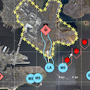
Lightspeed: display military symbology samples.symbology.lightspeed.MainPanel
This sample shows how to create, display, and edit military symbols on a map represented by a Lightspeed view. The sample allows switching between APP-6A, APP-6B, APP-6C, APP-6D, MIL-STD-2525b, MIL-STD-2525c, and MIL-STD-2525d. A few military symbols are already shown on the map.
Additionally this sample shows how to apply a clustering model and styler to an existing model. When zooming out, the sample will cluster identical symbols which not classified as part of the sea dimension.
Instructions
Click on a military symbol on the map to select it. You can drag the shape or its handles to edit the geometry, and change the properties and style in the symbol properties panel on the right.
New symbols can be made by typing in the name in the search box of the toolbar, or by clicking the browse button next to it. Next, click on the map to place the symbol at the desired location. Multiple clicks can be required depending on the type of symbol (line, area, arrow, ...); a right-click ends this step.
The star-shaped button in the symbol properties panel adds the symbol as a favorite in the toolbar, allowing rapid creation of this symbol.
Zooming out leads to the formation of clusters in order to keep the overview.
Lightspeed: all military symbols samples.symbology.lightspeed.allsymbols.MainPanel
This sample shows all military symbols in a Lightspeed view.
Instructions
The sample displays a layer with a number of symbols. The sample allows switching between
APP-6A, APP-6B, APP-6C, APP-6D, MIL-STD-2525b, MIL-STD-2525c, and MIL-STD-2525d. It also allows to switch between
icon symbols and tactical graphics.
Note that switching to tactical graphics might block the application for a moment, because of
the exceptional amount of complex strokes.
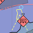
GXY: visualizing and editing Nato Vector Graphics (NVG) samples.symbology.nvg.gxy.MainPanel
This sample demonstrates how to decode, display, customize and edit NVG data in a GXY View. The sample decodes an NVG file illustrating a fictitious takeover of San Francisco. All military symbols in the file come from the APP-6B standard. For illustration purposes, some points use a domain specific symbol set to show civilian entities. The sample allows switching between APP-6A, APP-6B, APP-6C, APP-6D, MIL-STD-2525b, MIL-STD-2525c and MIL-STD-2525d.
The custom painter provider is a TLcdNVGGXYPainterProvider with a registered painter provider for the domain specific symbols. This painter provider is simply an icon painter.
Instructions
Click on a symbol on the map to select it. You can drag the shape or its handles to edit the geometry, and change the properties and style in the symbol properties panel on the right.
New symbols can be created by typing in the name in the search box at the top. Alternatively, click the browse button next to the search box, select the desired symbol, and click the create button. Optionally, you can change the supported geometry for the symbol on the left. Next, click on the map to place the symbol at the desired location. Multiple clicks can be required depending on the type of symbol (line, area, arrow, ...); a right-click ends this step.
You can save your changes by clicking the appropriate toolbar button.
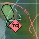
Lightspeed: visualizing and editing Nato Vector Graphics (NVG) samples.symbology.nvg.lightspeed.MainPanel
This sample demonstrates how to decode, display, customize and edit NVG data in a Lightspeed View. The sample decodes an NVG file illustrating a fictitious takeover of San Francisco. All military symbols in the file come from the APP-6B standard. For illustration purposes, some points use a domain specific symbol set to show civilian entities. The sample allows switching between APP-6A, APP-6B, APP-6C, APP-6D, MIL-STD-2525b, MIL-STD-2525c and MIL-STD-2525d.
The styler used in the sample styles NVG domain objects as defined in NVG by passing a TLspNVGStyle. For domain specific symbols, the styler passes a TLspIconStyle with a custom icon.
Instructions
Click on a symbol on the map to select it. You can drag the shape or its handles to edit the geometry, and change the properties and style in the symbol properties panel on the right.
New symbols can be created by typing in the name in the search box at the top. Alternatively, click the browse button next to the search box, select the desired symbol, and click the select button. Optionally, you can change the supported geometry for the symbol on the left. Next, click on the map to place the symbol at the desired location. Multiple clicks can be required depending on the type of symbol (line, area, arrow, ...); a right-click ends this step.
You can save your changes by clicking the appropriate toolbar button.
Infrastructure Standards

Converting BIM datasets to 3DTiles samples.bim.converter.BIMConverter
This is a command-line sample. Click More info for run instructions.
This command-line tool demonstrates how to decode BIM data (Binz, IFC, Revit, Navisworks) and export them as a 3DTiles dataset.
Run the sample using the shell script in the samples folder:
bim.converter.bat -i=<inputFile> -o=<outputPath>
The tool has two mandatory parameters: the path to the input BIM file, and the path of the output directory where the 3DTiles dataset will be written.
If you execute it with invalid or insufficient arguments, the tool prints out its usage documentation.
The supported data formats are Binz, IFC, Revit and Navisworks. Please refer to the respective documentation articles for more specific information about these formats.
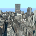
MeshUp CLI samples.meshup.Meshup
This is a command-line sample. Click More info for run instructions.
This command-line tool demonstrates how to use the 3D Tiles Processing Engine, which allows automatic tiling and multi-leveling of an OBJ dataset into a 3DTiles dataset. The produced tileset can then be optimally served by LuciadFusion.
Run the sample using the shell script in the samples folder:
meshup.bat -i=<input (OBJ) File or Folder> -o=<outputPath>
The tool has two mandatory parameters: the path to the the input OBJ file or folder containing OBJ files, and the path of the output directory where the 3DTiles dataset will be written.
If you execute it with invalid or insufficient arguments, the tool prints out its usage documentation.
For more information about MeshUp and its parameters, see the 3D Tiles processing Engine documentation page.
Maritime Standards
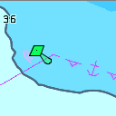
Lightspeed: displaying ECDIS data samples.decoder.ecdis.lightspeed.MainPanel
This sample demonstrates how to load and display ECDIS data on a map, and configure S-52 display settings interactively.
While this sample only demonstrates S-52 on a Lightspeed view, you can easily use the same approach on a GXY view.
The sample loads data using the registered ILcdModelDecoder services, and uses the registered ILspLayerFactory services.
In practice, this will be:
TLcdS57UnifiedModelDecoderto load S-57 catalogs and/or cellsTLcdS63UnifiedModelDecoderto load S-63 encrypted catalogs and/or cellsS52LayerFactoryto create Lightspeed layers with the S-52 symbology (delegates toTLspS52LayerBuilder)S52GXYLayerFactoryto create GXY layers with the S-52 symbology (delegates toTLcdS52GXYLayerFactory)
Both the GXY and Lightspeed layers can be configured with a TLcdS52DisplaySettings instance to configure the styling.
This sample provides a UI component to interactively change the S-52 display settings.
This sample supports
- S-57 and S-63
- ENC, AML and IENC
To load S-63 catalogs or cells, you need:
- The "S-63" Additional Component
- A license that has a User Permit (s63UserPermit tag) - tag is not necessary when loading the sample data (NO5F1615.000)
- A Cell Permit (ENC.PMT or PERMIT.TXT) corresponding to the User Permit, placed next to the input data
Instructions
The sample will automatically load an individual ENC cell and fit on it.
The S-52 display settings button can be used to display the S-52 display settings dialog. It allows to modify each individual S-52 display setting, supported by the S-52 rendering engine.
Objects can be double-clicked to see a list with their attributes.
The LuciadLightspeed distribution contains no multileveled ECDIS data. NOAA, the U.S. National Oceanic & Atmospheric Administration provides a large dataset on its website, which can be found at http://www.nauticalcharts.noaa.gov/mcd/enc/
The LuciadLightspeed distribution contains no AML data. UKHO, the United Kingdom Hydrographic Office, provides a sample AML dataset on its website, which can be found at http://www.ukho.gov.uk/Defence/AML/Pages/Home.aspx
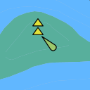
GXY: displaying S-101 data samples.decoder.s101.gxy.MainPanel
This sample demonstrates how to load and display S-101 data on a GXY view.
Data
This sample does not include any S-101 2.0 datasets by default. You may obtain suitable test data from the following sources:
- S-164 test data: https://github.com/iho-ohi/S-164-Sub-Group/tree/main/data/Staging/S-101/v2.0.0
- ENC FR_V2 test data: https://diffusion.shom.fr/expertises-formation/jeux-de-donnees-test-s-100.html
Explanation
This sample decodes complex geographical features defined in S-101 catalogs or cells and renders them using standardized symbology. It also intelligently manages when and how different layers of data are loaded and displayed, based on the user's selected S-101 display settings using the options panel in the sample's GUI.
The sample loads data using the registered ILcdModelDecoder services, and uses the registered ILcdGXYLayerFactory
services to create layers for the data.
In practice, this will be:
TLcdS101ModelDecoderto load S-101 catalogs and/or cellsS101GXYLayerFactoryto create GXY layers with the S-101 symbology
The GXY layer can be configured with a TLcdS101DisplaySettings instance to configure
the styling. This sample provides a UI component to interactively change the S-101 display settings.
Instructions
The sample will automatically load individual ENC cells and fit on them. If a Catalog file is being loaded, the loading of all the cells in the catalog will be done on demand. This mechanism provides better performance when dealing with large datasets by only loading and rendering the data that is necessary for the current view extent and zoom level.
Upon starting the sample, the S-101 display settings panel is displayed adjacent to the map panel in the sample application window. The settings panel allows to modify each individual S-101 display setting, supported by the S-101 rendering engine. The changes are applied in real-time to the displayed data. This allows users to customize the visualization of the S-101 data according to their preferences or requirements in the GXY view.
Objects can be double-clicked to see a list with their attributes. This feature is useful for users who want to inspect specific details about the geographical features displayed on the map.

Lightspeed: displaying S-101 data samples.decoder.s101.lightspeed.MainPanel
This sample demonstrates how to load and display S-101 data on a Lightspeed view.
Data
This sample does not include any S-101 2.0 datasets by default. You may obtain suitable test data from the following sources:
- S-164 test data: https://github.com/iho-ohi/S-164-Sub-Group/tree/main/data/Staging/S-101/v2.0.0
- ENC FR_V2 test data: https://diffusion.shom.fr/expertises-formation/jeux-de-donnees-test-s-100.html
Explanation
This sample decodes complex geographical features defined in S-101 catalogs or cells and renders them using standardized symbology. It also intelligently manages when and how different layers of data are loaded and displayed, based on the user's selected S-101 display settings using the options panel in the sample's GUI.
The sample loads data using the registered ILcdModelDecoder services, and uses the registered ILspLayerFactory
services to build layers for the data.
In practice, this will be:
TLcdS101ModelDecoderto load S-101 catalogs and/or cellsTLspS101LayerBuilderto build Lightspeed layers with the S-101 symbology
The Lightspeed layer can be configured with a TLcdS101DisplaySettings instance to configure
the styling. This sample provides a UI component to interactively change the S-101 display settings.
Instructions
The sample will automatically load individual ENC cells and fit on them. If a Catalog file is being loaded, the loading of all the cells in the catalog will be done on demand. This mechanism provides better performance when dealing with large datasets by only loading and rendering the data that is necessary for the current view extent and zoom level.
Upon starting the sample, the S-101 display settings panel is displayed adjacent to the map panel in the sample application window. The settings panel allows to modify each individual S-101 display setting, supported by the S-101 rendering engine. The changes are applied in real-time to the displayed data. This allows users to customize the visualization of the S-101 data according to their preferences or requirements in the Lightspeed view.
Objects can be double-clicked to see a list with their attributes. This feature is useful for users who want to inspect specific details about the geographical features displayed on the map.
Using ECDIS data from a LuciadFusion WMS in a GXY view samples.wms.client.ecdis.gxy.MainPanel
This sample demonstrates how to visualize ECDIS data from a LuciadFusion OGC Web Map Service (WMS) in a GXY view, taking into account custom display settings. Both S-52 and S-101 display settings are supported.
This sample requires a LuciadFusion WMS service supporting SLD-based S-52 or S-101 styling.
You can use the tabbed display settings panel on the right side of the map to tweak the display settings for an ECDIS WMS layer. When the WMS layer supports S-52 SLD styling, the S-52 tab is enabled and selected. When the WMS layer supports S-101 SLD styling, the S-101 tab is enabled and selected. The WMS client encodes the chosen display settings into an SLD extension, and embeds this SLD in the GetMap request that is sent to the server. The LuciadFusion WMS server then returns the ECDIS map data, rendered with the settings from the SLD.
Instructions
During startup, the sample tries to connect to a public LuciadFusion OGC WMS service (http://sampleservices.luciad.com/wms). Additionally, you can connect to other LuciadFusion WMS services through the URL panel.
Map interaction: the toolbar offers a set of actions to navigate on and interact with the map. This includes the ability to pan and zoom, to measure distances and to switch the projection. When the selection projection does not match the available projects in the WMS service, the data is automatically reprojected, fully transparent for the user.
S-52 and S-101 display settings: The tabbed panel right of the map allows to modify the S-52 and S-101 display settings. Any change to the settings immediately refreshes any loaded WMS layer by sending new GetMap requests to the WMS server with updated SLD styling settings.

Using ECDIS data from a LuciadFusion WMS in a Lightspeed view samples.wms.client.ecdis.lightspeed.MainPanel
This sample demonstrates how to visualize ECDIS data from a LuciadFusion OGC Web Map Service (WMS) in a Lightspeed view, taking into account custom display settings. Both S-52 and S-101 display settings are supported.
This sample requires a LuciadFusion WMS service supporting SLD-based S-52 or S-101 styling.
You can use the tabbed display settings panel on the right side of the map to tweak the display settings for an ECDIS WMS layer. When the WMS layer supports S-52 SLD styling, the S-52 tab is enabled and selected. When the WMS layer supports S-101 SLD styling, the S-101 tab is enabled and selected. The WMS client encodes the chosen display settings into an SLD extension, and embeds this SLD in the GetMap request that is sent to the server. The LuciadFusion WMS server then returns the ECDIS map data, rendered with the settings from the SLD.
Instructions
During startup, the sample tries to connect to a public LuciadFusion OGC WMS service (http://sampleservices.luciad.com/wms). Additionally, you can connect to other LuciadFusion WMS services through the URL panel.
Map interaction: the toolbar offers a set of actions to navigate on and interact with the map. This includes the ability to pan and zoom, to measure distances and to switch the projection. When the selection projection does not match the available projects in the WMS service, the data is automatically reprojected, fully transparent for the user.
S-52 and S-101 display settings: The tabbed panel right of the map allows to modify the S-52 and S-101 display settings. Any change to the settings immediately refreshes any loaded WMS layer by sending new GetMap requests to the WMS server with updated SLD styling settings.
Radar Connectors
Viewing ASTERIX Data Model samples.decoder.asterix.datamodelviewer.MainPanel
This sample shows the data model of all supported ASTERIX categories, for both tracks and trajectories.
This sample generates a list of data models trees. The data models contain all declared properties of all declared types inside the data model. The sample can generate strings for any given property, which can then be used in conjunction with a TLcdDataObjectExpressionLanguage to generate a value for a data object of the selected data type.
Instructions
Select data types on the top. This will generate a tree in the center of the frame. Each tree contains a list of properties. By clicking on a property, you generate a string that is visible in the textarea on the bottom of the frame.
A property itself also has a data type that in turn can have its own list of properties.
GXY: replaying recorded ASTERIX track or weather data samples.decoder.asterix.file.MainPanel
This sample shows how to decode an ASTERIX file and create a realtime presentation of this data.
This sample decodes an asterix file, which contains information in the form of trajectories. For each of these trajectories, a track is created that represents that trajectory at a certain point in time. This time can be controlled by the Simulator control panel at the bottom of the window.
Since ASTERIX data usually is relative with respect to a radar, the positions of the radars must be specified. These positions can be entered in the locations.cfg file. If you have your own ASTERIX data you wish to load, you will need to add the locations of your radars to this file.
Furthermore you can view the detailed properties of a track by double-clicking on it.
Each track is labeled with its track number when zoomed in. The labels avoid overlap in a continuous fashion by moving the labels around gently. In the event labels get mixed up, they can be dragged to a new location, after which they move back automatically.
Instructions
Press the "Open" button on the toolbar to open an ASTERIX file. Some sample data is available in the LuciadLightspeed distribution. If you have your own ASTERIX data you wish to load, you will need to add the locations of the radars to the locations.cfg file.
Click on an ASTERIX track to view the details on it in a popup.
You can use the controls at the bottom of the page to control the simulation:
- Press the Run button to start the simulation. The tracks will start moving.
- Press the Pause button to pause the simulation when it is running. The tracks will stop moving.
- Press the Stop button to stop the simulation. All tracks will be reset to their initial position.
- When the simulation is not running, drag the time slider to change the simulation time. The position of the tracks will be updated according to this simulation time.
- Change the "Speed-up" slider to change how much faster "simulation time" flows with respect to "real time". For instance, when set to 60, one minute of "simulation time" will tick by every second. Setting this value higher will make the tracks move faster.
Zoom in to see the labels of the tracks. After that you can move the text-labels by
- enabling the select controller in the toolbar
- moving your mouse cursor over one of the text-labels
- clicking and dragging the text-label
Lightspeed: visualization of ASTERIX category 240 radar video samples.decoder.asterix.lightspeed.radarvideo.MainPanel
This sample shows how to visualize an ASTERIX cat. 240 radar feed using TLspRadarVideoLayerBuilder. The sample uses a generated ASTERIX 240 data stream, which is sent to the decoder at a specified block rate. The stream is generated based on track data which is loaded from another ASTERIX file. It also contains some simulated noise, which can be filtered out using the styling panel (see instructions below).
Furthermore, the sample demonstrates the use of ALcdASTERIXReferenceProvider to supply the position of the radar platform, which is not included in ASTERIX category 240 data. Finally, it also illustrates the various styling options that are available for radar video layers.
Instructions
The styling of the radar layers can be configured using the controls in the bottom right panel. You can change the following properties of the styling:
- Colors: change the color of the background, sweep and blips.
- Afterglow duration in seconds: increasing this creates a "history trail" effect on the blips.
- Intensity: increasing this makes blips with a low amplitude stand out more.
- Threshold: the minimum amplitude required for a blip to be displayed. Increase this to filter out unwanted noise.
- Enable or disable the sweep and grid lines.
Creating a track display in Lightspeed view showing ASTERIX track data samples.decoder.asterix.lightspeed.trackdisplay.MainPanel
This sample shows how to visualize ASTERIX data on a track display.
Instructions
The sample shows a track display view, populated with tracks. Each track has a history trail and a label with some information in it. It is possible to hover over or highlight certain tracks by clicking on their icon. Once a track is highlighted, it is displayed using a different icon and it has more content in its label. Among this new content is a comments field which can be modified by clicking on it. Track labels can be moved by dragging them with the middle mouse button.
Track labels have the following content:
- Target address (Cat 21) or Track Number (Cat 62)
- Flight level
- Ground speed, in kilometers per hour
- Mode 3/A code (on hover or when highlighted)
- Custom text (on hover or when highlighted), can be modified when highlighted
In general, the implementation for the labels of this track display aims to keep labels as stable as possible. Zooming and panning should not affect the label locations, pin lines should not move when a track is highlighted, etc... This way, the sample tries to reduce noise as much as possible. This for example explains why labels can be only partially visible at the edge of the map.
GXY: visualizing live ASTERIX track or weather data samples.decoder.asterix.live.MainPanel
This sample shows how to create a live stream from an ASTERIX final file.
This sample will process the ASTERIX final file so that the ASTERIX live decoder can replay the data as if it were live data. The decoder will maintain a list of tracks and update them according to the information it receives from the live InputStream. As stated above, in this sample this live InputStream will be derived from a final ASTERIX file.
Since ASTERIX data usually is relative with respect to a radar, the positions of the radars must be specified. These positions can be entered in the locations.cfg file. If you have your own ASTERIX data you wish to load, you will need to add the locations of your radars to this file.
Each track is labeled with its track number when zoomed in. The labels avoid overlap in a continuous fashion by moving the labels around gently. In the event labels get mixed up, they can be dragged to a new location, after which they move back automatically.
When you double-click on a track, detailed properties will be shown in a popup.
Instructions
The sample opens a predefined ASTERIX file and starts replaying it.
Double-click on an ASTERIX track to view the details on it in a popup.
Zoom in to see the labels of the tracks. After that you can move the text-labels by
- enabling the select controller in the toolbar
- moving your mouse cursor over one of the text-labels
- clicking and dragging the text-label