Introduction
About Lucy
Lucy is an application component built with LuciadLightspeed that allows you to quickly load, display, explore, analyze, edit, and save geographic data. You can easily customize Lucy’s layout and user interface without any programming. It is possible to integrate Lucy with other applications (on the same host or another) with other libraries or even with other application frameworks such as Eclipse RCP and NetBeans.
You can install LuciadLightspeed components to add functionality to Lucy such as terrain analysis, trajectory preview and playback, and more. Lucy is deployed in, for example, applications for command and control, Air Traffic Control and Air Traffic Management (ATC/ATM), and the maritime sector.
The functionality discussed in this guide is available in all LuciadLightspeed product tiers.
About this guide
The purpose of this guide is to get the reader familiar with the functionality that Lucy offers out of the box, that is the functionality for which you do not need to program or configure anything. This guide provides a detailed description of Lucy’s default functionality and its extended functionality per LuciadLightspeed component. This guide is written for any end user of Lucy and although it does not require any specific knowledge to read it, the assumption is that the reader has a common understanding of applications for visualizing geographic data.
|
This user guide does not provide configuration or development guidelines. |
Main sections
The information in this guide is organized into the following sections:
-
Part I --- Default functionality: This part explains the default functionality of Lucy, that is the essential functionality that Lucy offers.
-
Part II --- Extended functionality: This part describes the functionality added to Lucy by installing additional LuciadLightspeed components.
Conventions
This section describes the typographical conventions and terminology for mouse actions that are used in this guide.
Typographical conventions
-
Bold text is used for names of GUI elements such as buttons, menu items and options, icons, and tools. Note that when the name is used multiple times in a paragraph, only the first occurrence of the name is bold.
-
The → sign is used for submenus as for example in Map→ Controls.
-
Reference text is used for internal references to sections, figures, or tables as for example in: Figure 1, “The default user interface of Lucy” shows the default user interface.
-
Typewritertext is used for file names.
|
Information paragraphs contain important information or useful tips. |
Terminology for mouse actions
The following terminology is used for the different mouse actions:
-
Click: click once with the left mouse button.
-
Right-click: click once with the right mouse button.
-
Double-click: click twice (quickly) with the left mouse button.
-
Drag: press the left mouse button while moving the mouse.
For a list of keyboard shortcuts that you can use in Lucy refer to Appendix C, Shortcut key combinations.
Contact information
If you have any questions after reading this guide you can contact the Luciad Support Desk services by mailing to support.luciad.gsp@hexagon.com or dialing +32 (0)16 26 28 30.
Default functionality
Getting started
This article tells you where to find the installation instructions for Lucy and explains how to start Lucy. In addition, this article introduces the elements of Lucy’s default interface, and provides basic instructions for working with maps, map objects and map data. Read this article if you are new to Lucy and want to get familiar with its concepts and terminology.
Installing and starting Lucy
If you used the automatic LuciadLightspeed installer to install your LuciadLightspeed distribution, Lucy was also installed on your system at that time.
To update your LuciadLightspeed installation with Lucy, unzip the Lucy zip file in the LuciadLightspeed installation folder.
|
Before starting Lucy, make sure that Java Runtime Environment 1.8 or later is installed on your computer. |
To start Lucy, click Lucy on the LuciadLightspeed launcher. You can start the LuciadLightspeed launcher by double-clicking start.jar in the LuciadLightspeed root directory.
To start Lucy without the launcher:
-
On a computer running Microsoft Windows, execute
Lucy.bat. -
On a computer running a Linux-based operating system, execute
Lucy.sh.
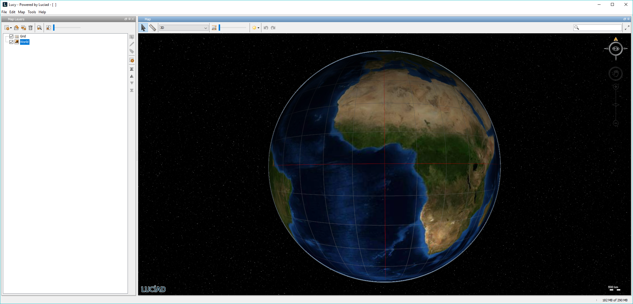
The Lucy interface looks as shown in Figure 1, “The default user interface of Lucy”. For a description of Lucy’s default user interface, refer to Exploring the default user interface.
Starting other Lucy types
You will notice that other varieties of Lucy are available on the LuciadLightspeed launcher and in the list of launch scripts: Lucy GXY and map-centric Lucy.
For a more in-depth explanation of all front-ends, see Choosing a Lucy frontend.
Lucy GXY
To start Lucy GXY, start the appropriate GXY equivalent script: LucyGXY.bat and LucyGXY.sh.
Those GXY scripts start up a GXY version of Lucy with a 2D map view, while the main Lucy options launch Lucy with a 3D map. In Lucy GXY, you can still start a 3D map alongside the initially launched 2D map.
|
Some of the functions discussed in the Lucy user guide may be specific to either Lucy or Lucy GXY. If this is the case, the function will be marked as such in the guide. |
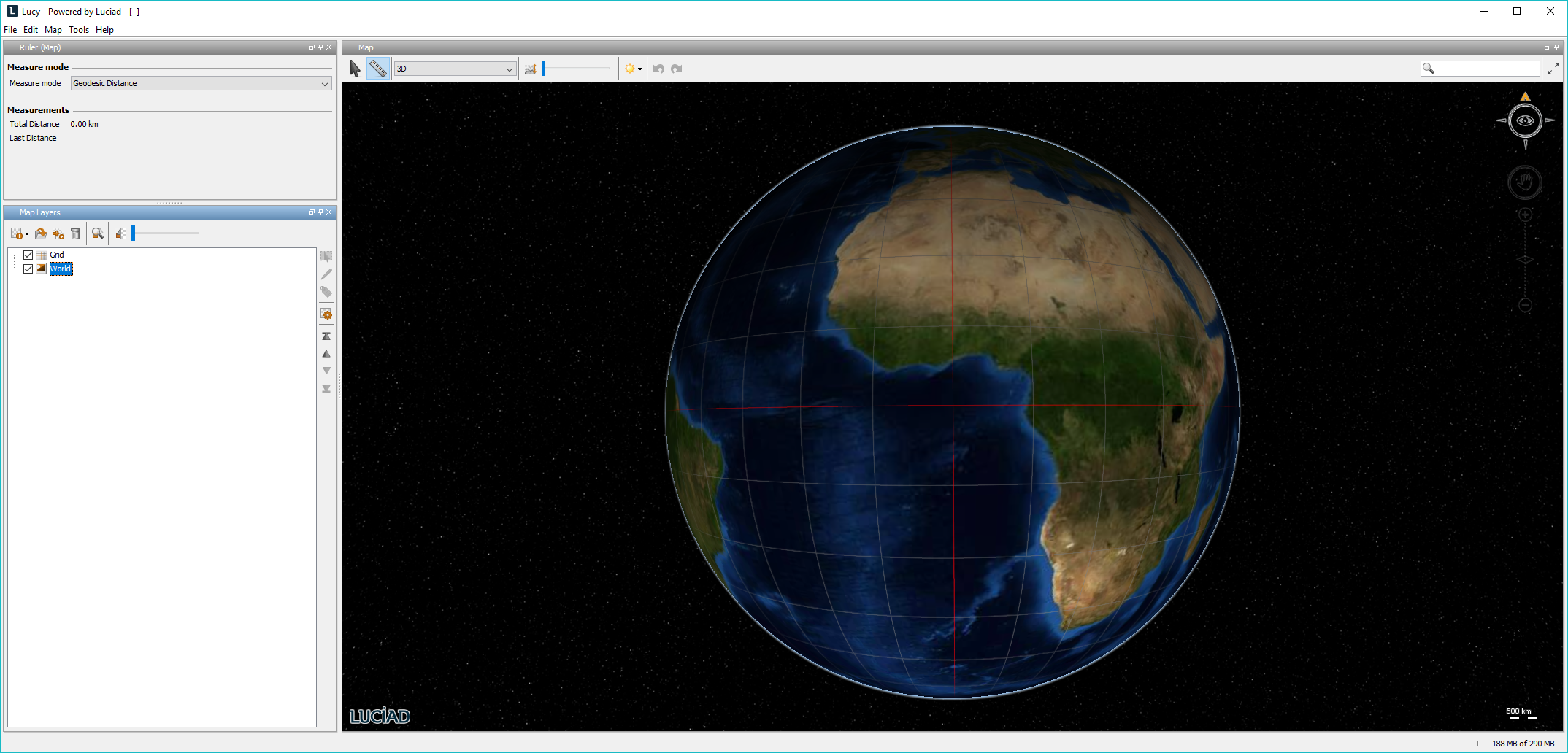
Exploring the default user interface
This section describes the elements of Lucy’s default user interface, without the installation of additional components. By default Lucy is started in an application window containing the following elements:
-
The title bar
-
The menu bar
-
The Map panel
-
The Map Layers panel
Lucy GXY also shows a Map Overview panel. It displays a visible map area as a cyan circle on a 3D globe. For more information about this panel, see [map_overview_gxy].
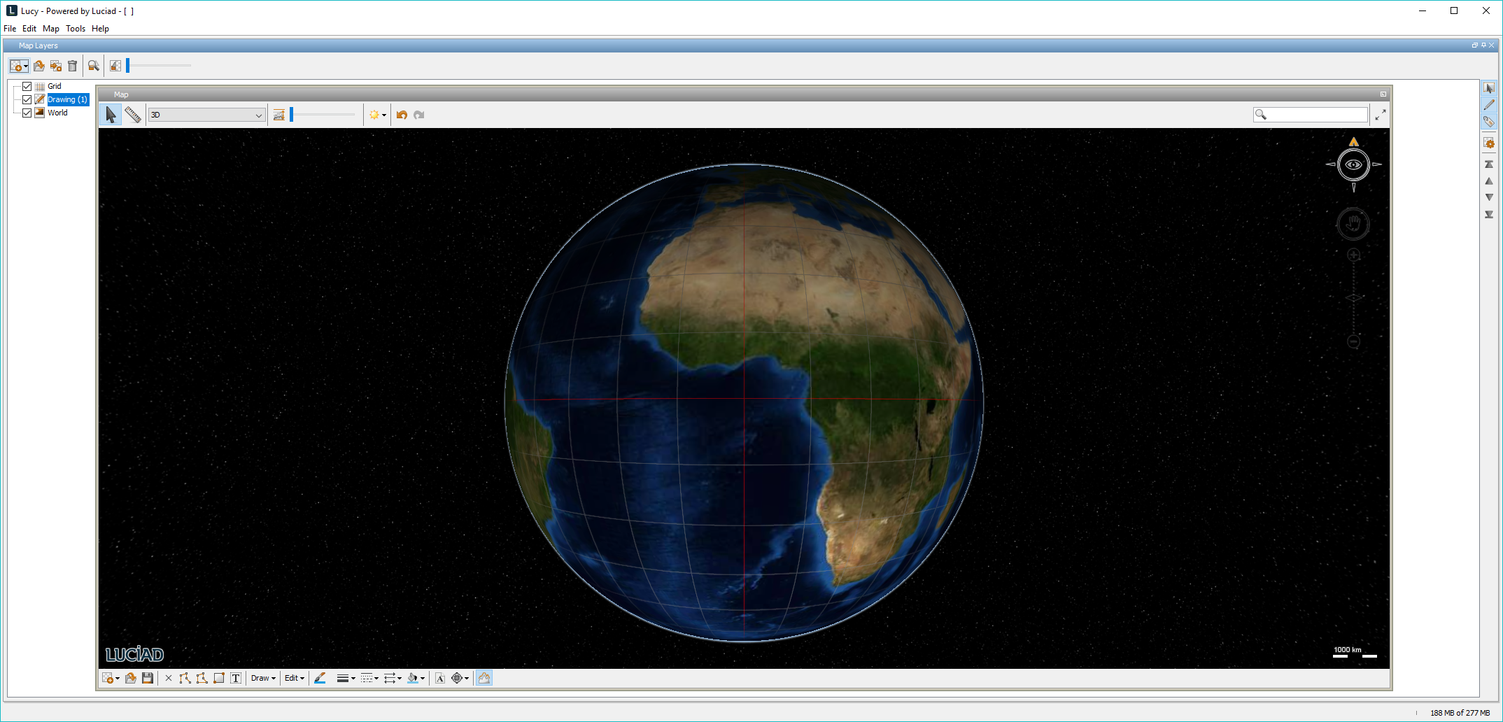
Figure 3, “The basic elements of Lucy’s user interface” shows the elements of Lucy’s default user interface.
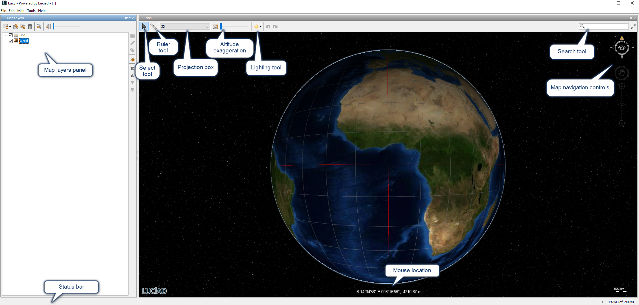
The title bar and status bar provide details on the application status. With the icons in the top right corner of the title bar you can minimize, maximize or restore, and close the application window.
The status bar also reports warnings and errors that occurred during data loading, for example. For more information, see Consulting warning and error logs.
Lucy’s default menu bar contains the menus File, Edit, Map, Tools, and Help. The Default functionality chapter of the Lucy user guide describe the tasks that you can perform with the default menus.
|
If you have installed extra LuciadLightspeed components, the menu structure of your Lucy application may differ from the default user interface. For more information on the functionality of each extra component and its effect on the user interface, refer to Extended functionality. |
The sections below provide a description of the different panels that appear in the default user interface.
The Map panel
The Map panel is the main panel in the Lucy application window and displays the loaded data in 3D. To open a map, select File→ New→ Map.
The basic elements of the Map panel are:
-
The title bar. The icons on the title bar allow you to show, hide, or restore the panel in the application window. Rearranging panels provides more information on the arrangement of panels.
-
The toolbar as described in more detail in The map tools.
-
The map view. This view displays the map data.
The Map layers panel shows the layers that are loaded to the map. By default the map contains a world layer and a grid layer. To learn how to use the Map layers panel, see Working with layers.
The map tools
The toolbar of the map, as shown in Figure 4, “The map toolbar”, allows you to interact with the map.

The toolbar of the map contains the following map tools:
-
 The Select tool to select objects on the map. This tool is activated by default. While it is active, you can also manipulate the map
view and viewing perspective. Working with maps, map objects and map data offers more information about working with maps and objects.
To select this tool from the menu, go to Map→ Controls → Select/Edit.
The Select tool to select objects on the map. This tool is activated by default. While it is active, you can also manipulate the map
view and viewing perspective. Working with maps, map objects and map data offers more information about working with maps and objects.
To select this tool from the menu, go to Map→ Controls → Select/Edit.
-
 The Ruler tool to measure distances on the map. The Ruler tool allows you to create a path on the map and measure distances of that path. When activating the Ruler tool, a Ruler panel
appears which allows you to change settings of the measurement mode and to view the measurements of the path. Measuring distances on the map describes the Ruler tool in more detail. To select this tool from the menu, go to Map→ Controls → Ruler.
The Ruler tool to measure distances on the map. The Ruler tool allows you to create a path on the map and measure distances of that path. When activating the Ruler tool, a Ruler panel
appears which allows you to change settings of the measurement mode and to view the measurements of the path. Measuring distances on the map describes the Ruler tool in more detail. To select this tool from the menu, go to Map→ Controls → Ruler.
-
The projection selection drop-down menu allows you to change the currently displayed map projection. For more information on the map projection, refer to Changing the map projection.
-
The Altitude exaggeration slider
 determines the scale for enlarging altitudes in the map view. By default, altitudes are not enlarged. To enlarge altitudes
in the map view, pull the slider towards the right.
determines the scale for enlarging altitudes in the map view. By default, altitudes are not enlarged. To enlarge altitudes
in the map view, pull the slider towards the right.
-
The Undo
 and Redo
  icons. For more information on undoing and redoing actions refer to Undoing and redoing actions.
-
 The Lighting icon lets you determine the position of the sun. Clicking the icon opens a panel with 3 options:
-
No lighting: no lighting scheme is set. The entire map is bright.
-
Automatic: the position of the sun is adjusted automatically based on the location of the camera.
-
Time of Day: allows you to specify the sun’s position the sun, by setting a time of day and a time zone.
For more information about the lighting options, see Controlling the light on your map (Lucy).
-
-
 This box allows you to find geographic coordinates, places and layer data on the map. For more information about the search
options, see Finding places and data on the map.
This box allows you to find geographic coordinates, places and layer data on the map. For more information about the search
options, see Finding places and data on the map.
-
 The full screen icon allows you to expand your map view so that it covers your screen. Click the icon again to return to
the regular application view.
The full screen icon allows you to expand your map view so that it covers your screen. Click the icon again to return to
the regular application view.
The Lucy GXY toolbar additionally contains the following tools:
-
 The Pan tool allows you to move the map around in the map view. Click on a location on the map to pan to that location. Keeping the
left mouse button pressed allows you to move the map around.. To select this tool from the menu, go to Map→ Controls → Pan.
The Pan tool allows you to move the map around in the map view. Click on a location on the map to pan to that location. Keeping the
left mouse button pressed allows you to move the map around.. To select this tool from the menu, go to Map→ Controls → Pan.
-
 The Recenter tool allows you to change the center of the current map. Clicking on the map will recenter the map to the clicked position.
Use this tool for example to avoid distortion of the projection of the area of interest. To select this tool from the menu,
go to Map→ Controls → Center Map.
The Recenter tool allows you to change the center of the current map. Clicking on the map will recenter the map to the clicked position.
Use this tool for example to avoid distortion of the projection of the area of interest. To select this tool from the menu,
go to Map→ Controls → Center Map.
-
 This box displays the scale of the map. For more information on setting the map scale, refer to Changing the scale of the map.
The map navigation controls
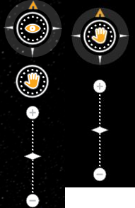
The map navigation controls help you move around on the map. Figure 5, “Lucy navigation controls and 2D Lucy GXY navigation controls” shows that the navigation controls for Lucy maps and 2D Lucy GXY maps are very similar.
Move the mouse over the controls to:
-
Move the map: to determine the direction click on the compass border surrounding the hand icon and keep the left mouse button pressed to move the map into the selected direction.
-
Rotate the map Click outside the compass center, in the area of the compass arrows, and drag the mouse into the rotation direction. To reset the map with the north up, click on the north arrow.
-
Change viewing perspective Click inside the compass icon and drag the mouse into the desired direction to tilt the map.
-
Zoom out of the map: click on the plus icon, keep the left mouse button pressed for continuous zooming.
-
Zoom in on the map: click on the minus icon, keep the left mouse button pressed for continuous zooming.
On 2D maps in Lucy GXY, there is just one navigation control icon to move and rotate the map, while you can use two separate controls on 3D maps.
|
The navigation controls are shown by default on the map. To hide the controls, deselect the Map→ Show Navigation Controls menu item. |
The mouse location
The location of the current mouse position is displayed at the bottom of the map by default, as shown in Figure 3, “The basic elements of Lucy’s user interface”. The mouse location is given in the specified coordinate system. To change the coordinate system and format, select Edit→ Point Format. To hide the mouse location, deselect the Map→ Show Mouse Location menu item.
The Map Layers panel
By default the Map Layers panel appears bottom left of the Map panel and shows the layers of the current map. If the Map Layers panel is not visible, select the Tools→ Layer Control menu item. Deselect the menu item to close the Map Layers panel. Figure 6, “The Map Layers panel” shows the Map Layers panel of the default map.
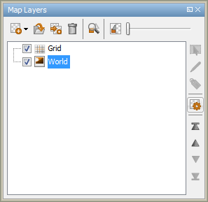
Working with layers provides detailed information on working with layers and using the Map Layers panel.
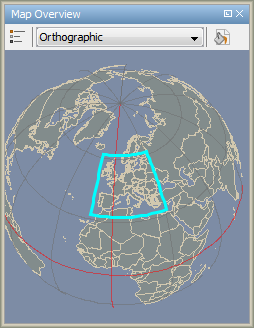
The Map Overview panel (Lucy GXY)
By default, the Map Overview panel is located top left of the Map panel. If the Map Overview panel is not visible, select the Tools→ Map Overview menu item. Deselect the menu item to close the Map Overview panel. The Map Overview shows outlines of the opened maps. It gives an overview of the maps and allows quick navigation by editing the map outlines. When multiple maps are opened, you can click on one of the map outlines in the Map Overview to see the name of the corresponding map. Figure 7, “The default Map Overview panel” shows the default Map Overview panel. Getting a map overview (Lucy GXY) describes the Map Overview panel in more detail.
Working with maps, map objects and map data
This section discusses how to move around and manipulate maps and objects. It also tells you where to find more information about loading and working with data. Finally, it provides an overview of the data formats you can load in Lucy.
Moving around on the map
To move around on the map, you can either use the navigation controls, as explained in The map navigation controls, or the computer mouse.
-
Move the map click on the map and drag the mouse. You can also press the middle mouse button down and move the mouse. On 2D maps in Lucy GXY, you must activate the pan tool before you can move the map.
-
Change viewing perspective right-click on the map and drag the mouse into the desired direction to tilt the map.
-
Zooming in and out on the map: click the map and scroll the middle mouse button up or down.
Working with objects on the map
|
You can select objects only if the corresponding layer is Selectable. You can edit objects only if the layer is Editable as described in The layer tools and options. |
When the select tool is active, you can:
-
Select an individual object click the object.
-
Select multiple objects shift-click the objects or drag a rectangle around the objects.
-
Delete objects right-click the objects and select the Delete menu item .
-
Show the properties of one selected object right-click the object and select the Properties menu item. The Object properties panel appears top left of the map as described in Changing the shape properties
-
Select an object from overlapping objects Alt-click the overlapping objects and select the required object from the menu
-
Deselect one object shift-click the object
-
Deselect all objects click a location on the map outside the selected objects
-
Move a selected object drag it to another location
-
Edit a selected object Ctrl-click the object
The color of Lucy objects changes once they are selected. You can change the colors applied to these selected objects. To change the fill, line, text or icon color of selected objects, go to Map→ Style settings… and open the Selection colors… tab. You can only change the object selection color on 3D maps, and not on 2D maps in Lucy GXY.
Working with data in maps
When you have opened a map, you can:
-
Load and save data as described in Loading and saving map data. Appendix A, Supported data formats describes the supported file formats.
-
Load and save workspaces as described in Loading and saving workspaces.
-
Work with the map layers as described in Working with layers. To add layers from other maps to the current map, use the Copy layers from another map icon
 in the layer control of the current map, as described in Copying layers from another map
 -
Work with multiple maps as described in Working with multiple maps. In Lucy GXY, you can choose between opening a new 2D map or 3D map by selecting the corresponding File→ New menu item.
-
Draw shapes, as described in Drawing shapes on the map.
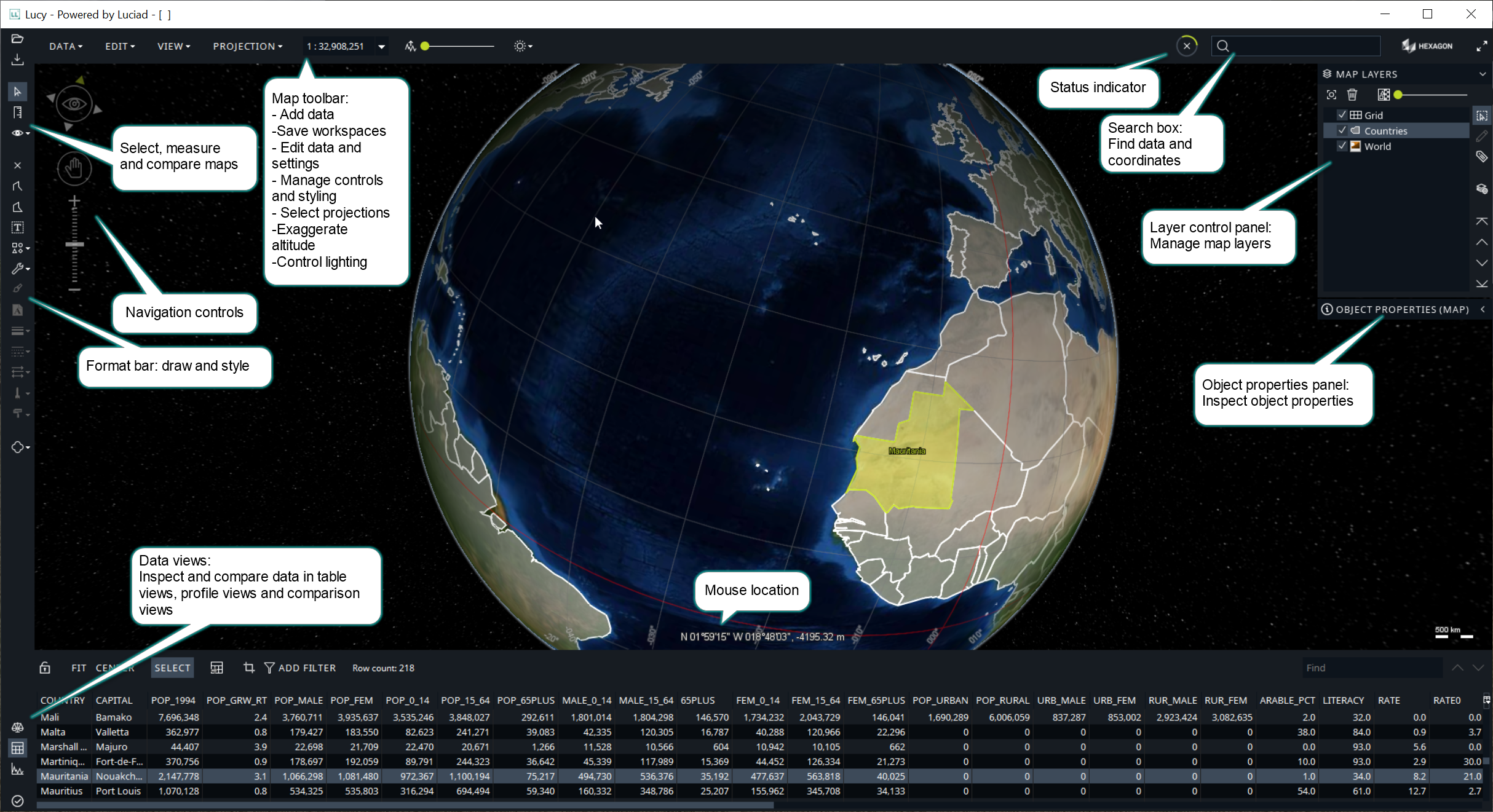
Exploring the map-centric user interface
This section describes the elements of Lucy’s map-centric user interface without extra components installed. By default, map-centric Lucy is started in an application window containing the following elements:
-
The title bar, including the icons to minimize, maximize and restore the application window.
-
The map as the central part of the application.
-
A top tool bar, providing access to overall functions and settings, such as data loading, general view settings, a status indicator for data loading, and search.
-
A side tool bar, containing the tools to add and manage map views and map objects, such as a drawing bar, comparison tools, and additional view options.
-
The Map Layers panel
-
The object properties panel.
The first time you start Lucy map-centric, the application will overlay the window with a user onboarding layer, to show first-time users where to find the main functions of the application. If you want to see this layer again at a later stage, press Shift+F1.
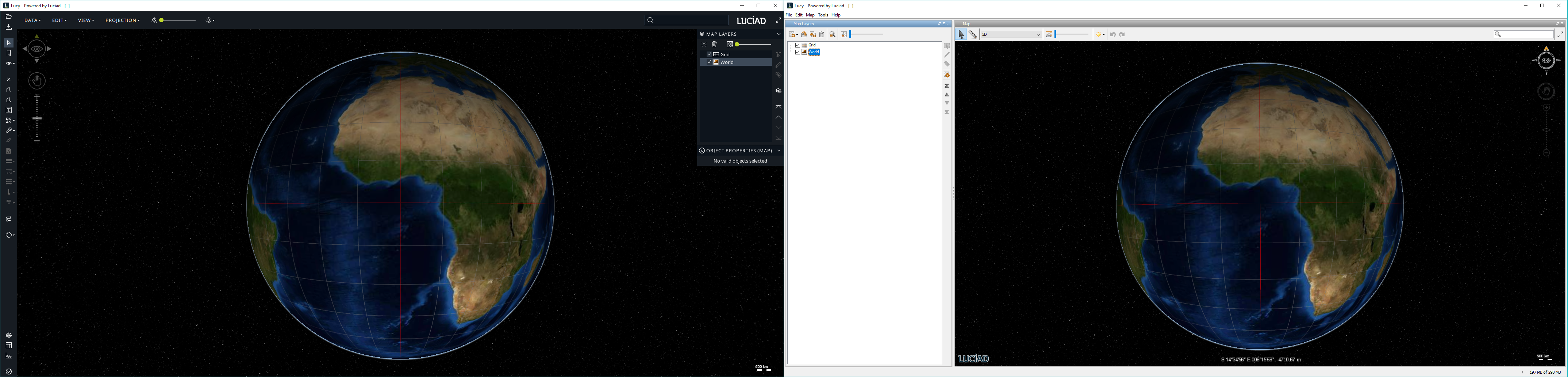
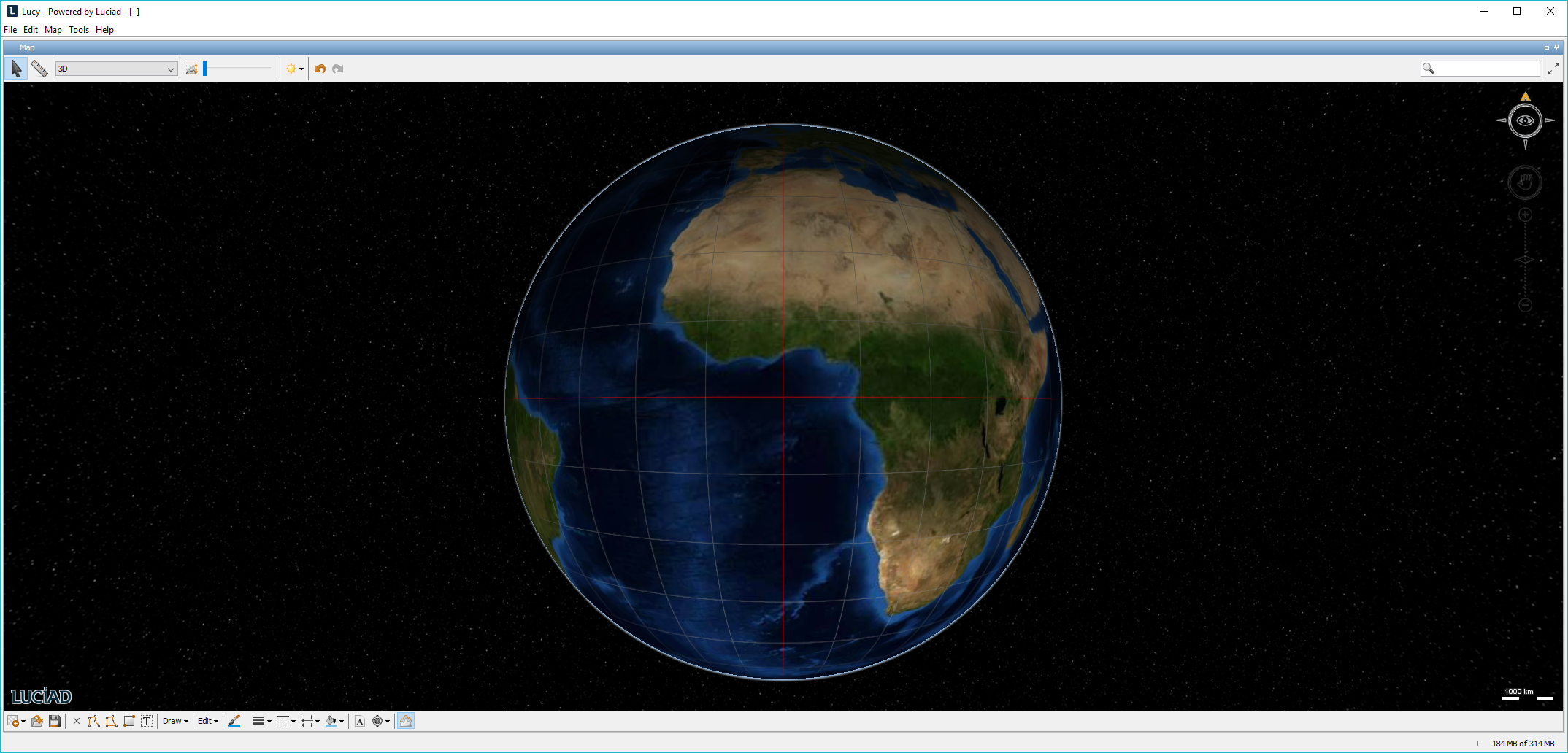
Figure 8, “The basic elements of the map-centric user interface” shows the elements of Lucy’s map-centric user interface.
The two additional buttons at the top of the side tool bar provide shortcuts for data loading:
-
 allows you to select and load a file in Lucy map-centric.
-
 allows you to enter a web service URL, and connect to data offered by a web service.
If you prefer to access all options through a typical menu bar, press F2 to visualize the default Lucy menu bar. The Default functionality section of the Lucy user guide describes the tasks that you can perform with the default menus.
|
If you have installed extra components beside Lucy, the tool bars of your map-centric Lucy application may contain more items. |
Customizing the user interface
This article provides information on how to change the appearance and behavior of Lucy’s default user interface and adapt it to your needs without programming or editing configuration files.
Changing the map name
To change the map name displayed in the map title bar, select Map→ Change name…. A dialog box opens that allows you to type in a new name.
Changing the look and feel
To quickly change the colors and fonts used for the panels, menus, and other elements in the interface, select the Edit→ LookandFeel menu item. The following options are available:
-
GTK (Linux only)
-
Metal
-
Nimbus
-
CDE/Motif
-
Windows (Windows only)
-
Windows Classic (Windows only)
|
Lucy uses third party software for some of these options. Restart Lucy after changing the look and feel to make sure that the third party implementations change all aspects of the selected look and feel. |
In addition, you can change the colors of each of the individual map layers as described in The layer paint style.
In Lucy GXY, you can also change the background color of a 2D map as described in Changing the map background color (Lucy GXY).
Rearranging panels
By default Lucy is started in docking mode which means that you can drag the panels and drop them to another location in or outside the main application window. The docking functionality allows you to arrange the panels to your preferences, for example to position a panel outside the main application window on a second screen.
Click in the title bar of the panel and drag the panel to:
-
The left part of another panel to move it to the left of that panel
-
The right part of another panel to move it to the right of that panel
-
The center of another panel, or to its title bar, to place the panel on top of the other panel
While you are dragging the panel, a frame is displayed to indicate the new location of the panel. Release the left mouse button to drop the panel to the location of the frame.
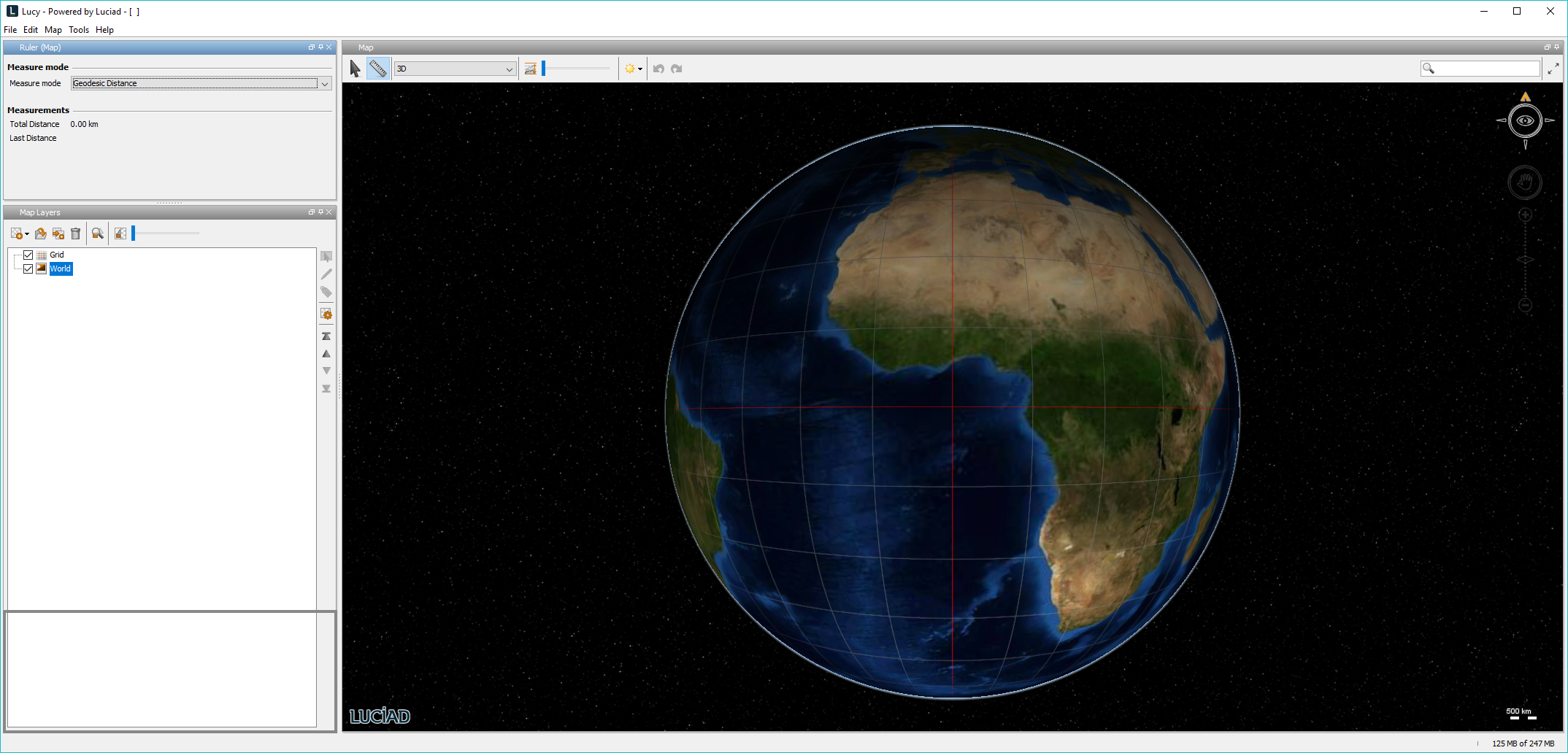
The following example shows how to move a panel to a new location. Figure 9, “The Ruler panel is on top of the Map layers panel” shows the default Lucy user interface with the Ruler panel on top of the Map layers panel.
To move the Ruler panel under the Map Layers panel, drag the panel until the frame is in the correct location as shown in Figure 10, “The frame showing the new location of the panel”.
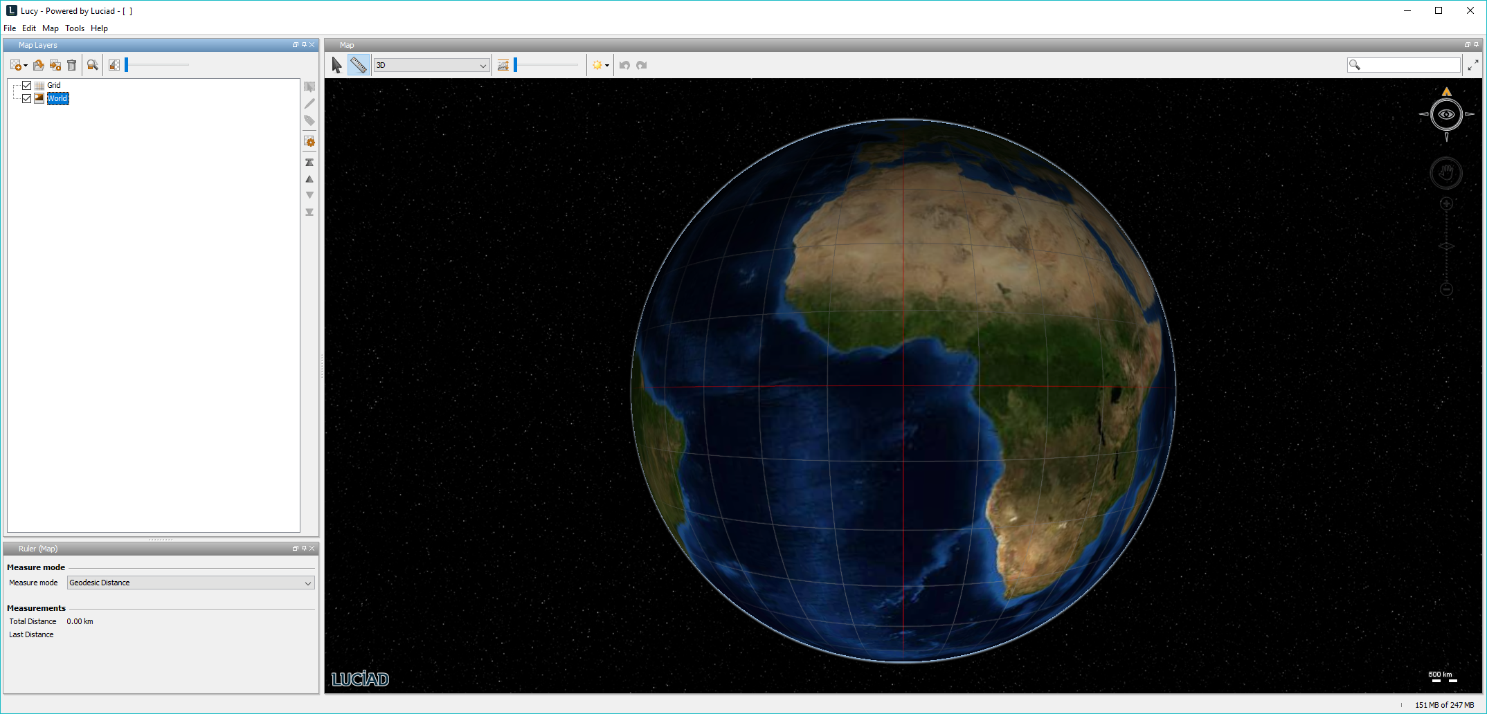
Finally, drop the panel to the frame and the panel is docked to its new location as shown in Figure 11, “The Ruler panel is under the Map Layers panel”.
Other ways of rearranging panels are available by right-clicking on the title bar of a panel. A menu pops up with the following options:
-
Close --- Select this option to close the panel. Note that at least one map panel needs to be open. You can also click on the Close icon in the title bar to close the panel.
-
Floating --- Select the Floating option to undock a panel and make it floatable so you can move it around inside or outside the application window (for example to display it on a second screen). If you deselect this option, the panel is docked to its original location. The Toggle floating icon on the title bar offers the same functionality. Figure 12, “A floating map panel” shows the application window with a floating map panel.
-
Auto Hide --- Use this option to hide a panel or press the Toggle auto-hide icon in the title bar. A hidden panel is minimized and shown as a tab located in one of the corners of the application window. To show a hidden panel, move the mouse over the panel tab. To deactivate the Auto Hide function, deselect the Auto Hide option from the pop-up menu or press the Toggle auto-hide icon. Note that you cannot hide all panels, at least one map panel needs to be open.
-
Maximize/Restore --- Use this option to maximize a panel and display it in the full application window. Restore the panel to its previous size by selecting the Restore option. The same functionality is available by double-clicking on the title bar. Figure 13, “A maximized map panel” shows the application window with a maximized map panel.
-
Reset layout --- Use this option to restore the panels according to the last saved workspace settings as described in Loading and saving workspaces.
|
To quickly maximize the Map panel to full screen, either press F11 or select Map→ Full screen. |
Resizing panels
To resize panels, select the division line between two panels. Move the mouse between the panels until the cursor changes
into a shape with arrows left and right, then click to make the division line visible. Drag the division line to resize the
panel. If a panel becomes too small to display all contents of the toolbar, an icon is added at the right side of the toolbar.
Click on the icon ![]() to add the missing content in a box under the toolbar.
to add the missing content in a box under the toolbar.
Changing the HTTP proxy settings
With Lucy you can load data from a web server, for example through the OGC protocols. In case you need to connect to one or more web servers with a web proxy, you can configure the settings by selecting Edit→ Proxy settings…. The Proxy settings dialog box appears as shown in Figure 14, “The Proxy settings dialog box”.
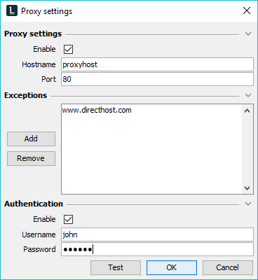
In the Proxy settings dialog box you can configure the following settings:
-
Proxy settings:
-
Enable: activate the use of a web proxy. If a web proxy is not enabled, the other options are not available.
-
Hostname: IP address or hostname of the web proxy.
-
Port: port of the web proxy. This is 80 by default.
-
-
Exceptions: use the Add and Remove buttons to create a list of hostnames that are reachable without proxy. Note that this option is collapsed by default if the list is empty.
-
Authentication:
-
Enable: activate authentication for the proxy server.
-
Username and Password: the credentials for the proxy server. Note that these options are collapsed by default if authentication is disabled.
-
You can use the Test button to verify if you can connect to one of the web hosts.
|
Note that these proxy settings apply to the entire Lucy application. |
- Map-centric Lucy
-
To configure your proxy settings in map-centric Lucy, go to Edit → Proxy settings….
Working with data
This article describes how to work with maps, workspaces, and layers and provides the basic knowledge needed for loading, visualizing, and saving data with Lucy.
Loading and saving map data
Loading map data
There are multiple ways to load data to the current map:
-
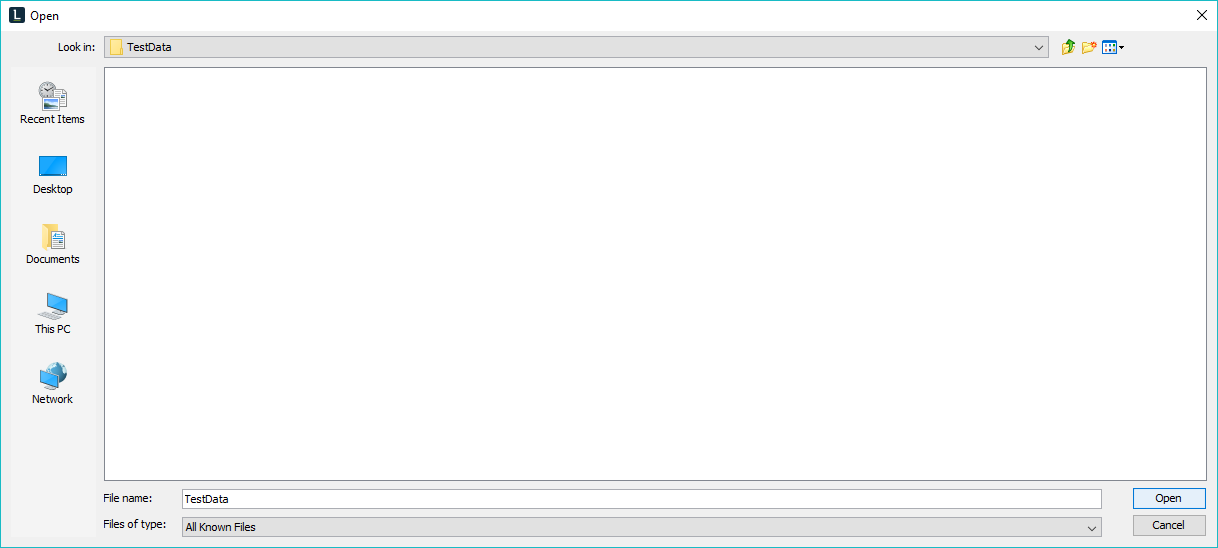
Select the File→ Open menu item. A dialog box pops up allowing you to select the files from which to load data. Figure 15, “The Windows dialog box to open files” shows the Windows dialog box for opening files. Keep the Ctrl-key pressed to select multiple files from the list with the left mouse button. A warning message appears when a file cannot be loaded in the current map. If another map is open, and can load the file, a dialog box appears that allows you to select the map and load the file.
-
Drag and drop files from the file list of your operating system, for example from a Windows explorer window, directly onto the map view.
-
Copy data layers from another map as described in Copying layers from another map.
- Map-centric Lucy
-
To load data on a map in map-centric Lucy, go to Data → Open…, or click the File icon in the top left corner of the application. You can also drag and drop files from the file list of your operating system.
Appendix A, Supported data formats shows the file formats and corresponding file extensions that Lucy supports. To add support for some of the file formats, you need to install extra LuciadLightspeed components.
|
You may have to select a georeference at this point. See Choosing a georeference for loaded map data for more information. |
The loaded data files are added to the map and to the Map Layers panel. The busy icon ![]() in front of a layer indicates that not all data for that layer has been loaded yet. You can continue with your operations
as the data is loaded in the background.
in front of a layer indicates that not all data for that layer has been loaded yet. You can continue with your operations
as the data is loaded in the background.
Click on the Fit to layer button or double-click on the newly added layer to fit the map view to the layer data. Use the icons on the right hand side of the layer list to change the order in which the layers are rendered in the map view. Working with layers describes how to work with layers.
Choosing a georeference for loaded map data
A prerequisite for the correct display of data on a map is the availability of georeference information for that data. The
georeference is the coordinate reference system associated with a set of map data. Usually, that information is either loaded
with the map data, or stored in a separate file alongside the data file by the map data provider. For example, a .shp file typically comes with a .prj file of the same name, which stores the georeference.
If you load a data file with an unknown georeference system, for example a .shp file without a .prj file, the Choose geo reference dialog pops up when you try to load the file. This dialog box allows you to select or define the georeference system. To
learn more about the contents of the dialog box, see Specifying the georeference system.
|
The map data provider determines the coordinate reference system. To know which georeference you have to select, first try and find out from the file collection offered by the data provider. The map data may come with a document that details the georeference. If you cannot find the georeference information, contact your map data provider. |
To save the georeference system you selected in a file in the directory of the data, select the Auto save check box in the bottom left corner of the dialog box. When you click OK, Lucy stores the reference file, and loads the data. The reference file gets the same name as the data file, and an .epsg, .prj, or .ref file extension. When you open the data file afterwards, the reference file is opened as well.
Loading styling and filtering information
Data files may come with companion style files, stored in the same folder as the data files. Such style files can define what
the data should look like on the map, and possibly if the data should be filtered for visualization. Lucy automatically picks
up and applies style files with .sty or .sld extensions:
- .sty files
-
Lucy-specific style files. For more information about creating
.styfiles, see The layer style file. - .sld files
-
files are styling and filtering files defined in the SLD/SE styling language developed by OGC. Note that
.sldfiles are not picked up on 2D maps in Lucy GXY.
Loading delimited data
Delimited data is table-like data that typically comes in the form of Comma-Separated Value (.csv) files. Each line in the file represents a data record. Each data field or column in the line is separated from the other with a delimiter such as a comma, a semi-colon, or a tab. Data separated by tabs may come in a Tab-Separated Value (.tsv) file. In some files, the first line serves as a table header row that identifies the data fields in the other lines.
If you want to load CSV files in Lucy, geospatial information is required, such as the required geometries and their coordinates. That information allows Lucy to visualize and position the data on the map. It is typically made available in the CSV file itself, or in a companion file.
To load a CSV file in Lucy, you can open it like any other file. Lucy automatically configures the settings for correctly loading the CSV file. To allow you to confirm or change those CSV loading settings, Lucy shows you a preview of the configuration result:
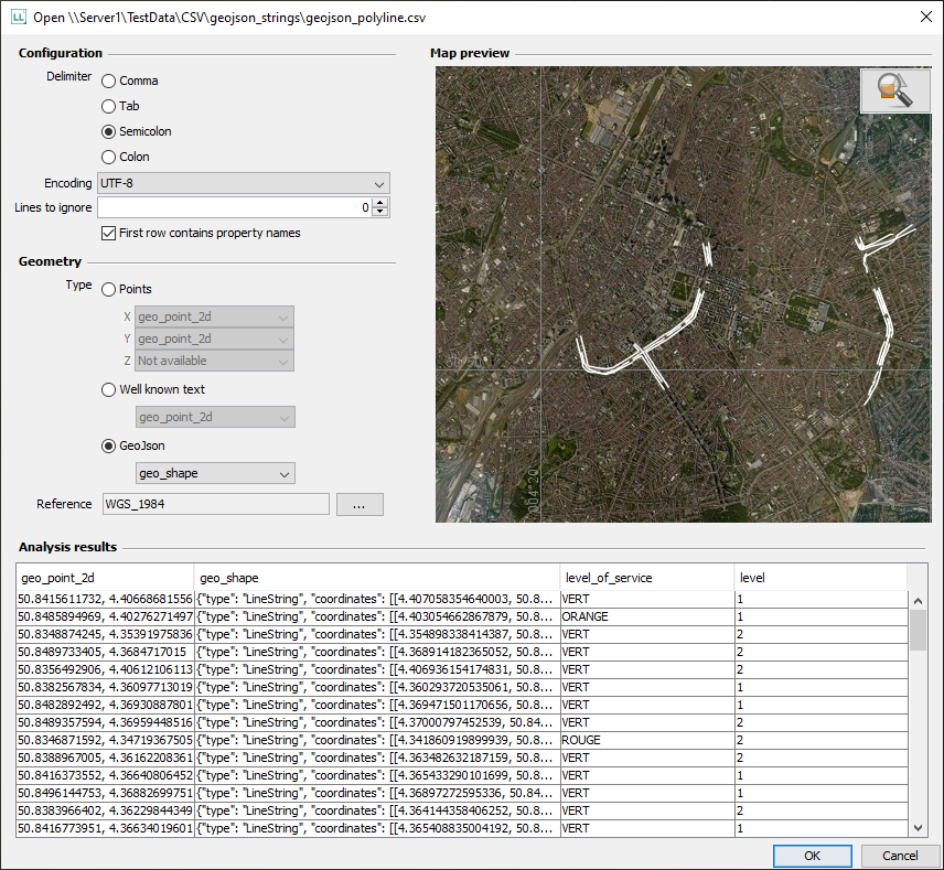
- Delimiter
-
Select the right delimiter from the radio button list if your file values are separated by another delimiter than the one determined by Lucy.
- Encoding
-
The encoding standard used in your CSV file.
- Lines to ignore
-
If the first few lines in your file are empty or contain irrelevant information, you can specify the number of useless lines here. As a result, Lucy skips that number of header lines during decoding. If the first file line contains data field names instead of values, select the check box below instead.
- First row contains property names
-
Select this check box if the first file line contains property names, and the rest of the file contains actual values.
- Geometry
-
Your CSV file can consist of:
-
Points with the X, Y and Z coordinates stored in specific columns
-
Well known text: the shapes in your CSV file may be specified in Well-known Text (WKT) markup language. The WKT string will include the shape coordinates and be stored in one specific column.
-
GeoJson: the shapes in your CSV file are specified in the GeoJSON format. The GeoJSON notation will include the shape coordinates and be stored in one specific column.
If Lucy has not determined correctly how the geometries are specified, or which column contains the specification, you can correct that here.
-
- Reference
-
Lucy needs georeference information to correctly position data on the map. CSV files usually do not contain any information about the coordinate reference system associated with the map data. Therefore, Lucy selects WGS84 as the default georeference. If another reference system applies, you can select it by clicking the button next to the text field. For more information, see Choosing a georeference for loaded map data. Lucy saves that georeference information as a .prj file next to your CSV file, so that you do not have to provide it again.
You can assess the effect of the settings in the Table preview as well as on the Map preview. Both previews update automatically if you change the settings.
When you are satisfied with the data previews, click OK to display your CSV file as a map layer.
|
To help Lucy determine the right data type for each column, you can create a CSVT (.csvt) companion file, and store it in the same folder as the CSV file. Lucy automatically picks up those files along with the CSV file itself. For more information about CSVT companion files, see http://www.gdal.org/drv_csv.html and https://giswiki.hsr.ch/GeoCSV. |
Saving edited map data
If you have edited map data you can save the changed data by selecting the File→ Save As menu item. A dialog box pops up in which you can select the layer from which you want to save the current data. After selecting the layer a dialog box appears that allows you to choose the format, the name, and the location of the file to save the data to.
- Map-centric Lucy
-
To save edited map data in map-centric Lucy, go to Data → Save Layer…, and select the layer of which you want to save the data.
Saving vector data
By default, you can save vector data to one of the following vector file formats:
-
Drawing
-
GeoJson
-
MIF
-
SVG
-
Shape
|
Keep in mind that if you load vector data in one format, and then save it to another format, not all of the original shapes may be saved in the new format. |
Saving raster data
The default raster format is GeoTIFF. The GeoTIFF format provides a few settings to optimize the output file:
-
Format: choice to save raster data either in the TIFF format or in the BigTIFF format. The BigTIFF format is a variant of the GeoTIFF format, without the 4 GB file limit usually applicable to GeoTIFF files. You can select the BigTIFF format to store a large amount of raster data in a file.
-
Compression: deflate (lossless compression, most suitable for vector drawings), JPEG (lossy compression, most suitable for imagery), and none (sometimes required for interchange with simple third-party tools).
-
Level count: the number of levels of detail to be precomputed and stored in the GeoTIFF file. Multiple levels of detail can significantly improve the performance when working with the resulting file, especially when zoomed out. The number of levels should generally be sufficiently large, such that the smallest level of detail measures only a few pixels in both dimensions.
-
Quality: the quality of the JPEG compression, if applicable.
-
Scale factor: the scale factor (in both dimensions) between subsequent levels of detail.
-
Tile height and tile width: the internal tile size, expressed in pixels. Internal tiling can significantly improve the performance when working with the resulting file, especially when zoomed in. Lucy only decodes the tiles that are actually visible, thus requiring less computation time and less memory.
To add support for other file formats you need to install additional components as described in Appendix A, Supported data formats.
Encoding JPEG 2000 files
You can use Lucy to write JPEG 2000 files. You can save part of a map as an image in the JPEG 2000 format, using the File→ Save As Image menu. A dialog box opens in which you can specify the following settings:
-
Compression: compress the file without data loss (lossless) or with some data loss (lossy)
-
Quality: the quality of the encoded image (where 1 is the best quality)
-
Quality layers: the number of quality layers (used for progressive decoding)
-
DWT levels: the number of Discrete Wavelet Transform levels. Best value indicates that the DWT levels are computed automatically depending on the tile or image size.
-
Tile height: the height of a tile in pixels
-
Tile width: the width of a tile in pixels
Loading KML data
KML is an XML-based file format for exchanging geographic annotations and visualizing them in Earth browsers. It was originally developed by Keyhole, Inc. as part of their Earth Viewer application, which is currently known as Google Earth. The KML file format was designed to be flexible and customizable. It allows content providers to store a wide variety of vectorial shapes and raster data, as well as dynamic behavior, external resources, visualization and temporal information. LuciadLightspeed officially supports KML version 2.2, though given the backward compatibility of the KML file format, a large subset of files that are of version 2.0 and 2.1 are also supported.
The KML 2.2 format
You can load KML 2.2 data using the File→ Open menu. The loaded data is displayed in the map view and the corresponding layers are added to the layer tree.
To view the properties of an KML 2.2 geometric object, select the object on the map, right-click and select Properties. The Object properties panel appears in the top left corner of the application window. The properties tree follows the XML structure of the selected object and allows you to view the available properties or all properties of the object.
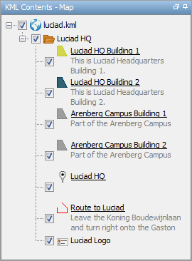
When you load KML 2.2 files, Lucy displays a KML Contents - Map panel. The content tree in the panel represents the underlying structure of all loaded KML files. Figure 17, “A KML content tree in the KML Contents - Map panel” is an example of such a KML content tree. You can double-click a tree node to fit the map view to that node. To change the visibility of a node, click on the check box next to it.
|
For a KML 2.2 object to be visible, its visibility check box must be selected in the KML Contents - Map panel. All its parent nodes must also have their visibility check boxes selected. |
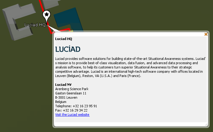
Some KML 2.2 objects have informative balloons attached to them. Figure 18, “A KML 2.2 balloon” shows an example of such a balloon. To display the balloon of an object, select the object in the view. You can also click on a node in the KML content tree. Balloons only get activated if the map has a single selection. When multiple objects are selected, no balloons will be displayed.
Balloons can be interacted with in the following ways:
-
Close a balloon by clicking the Close button in the top right corner of the balloon.
-
Move around the balloon by clicking and dragging the edge of the balloon.
-
Resize a balloon by clicking and dragging the Resize button in the lower right corner of the balloon.
|
Not all KML 2.2 objects have balloons. Objects without balloons will not display a balloon when they are selected. |
Some KML 2.2 files contain time-dependent data. Files that have time-dependent data will automatically be added to the Previewer panel. Using the Previewer provides more information on the Previewer panel and the simulation of data in real-time.
Loading LIDAR data
Lucy allows you to load and display Light Detection and Ranging (LIDAR) data from files in the LASer or E57 formats. These
files contain large numbers of points. The LASer formats typically have a .las or .laz (LASZip) extension, and the E57 format has an .e57 extension. These collections of points in LIDAR files are also referred to as point clouds. The LAZ files in particular can
contain a large number of points.
|
If the number of points in the file exceeds a certain threshold, Lucy will evenly reduce the loaded point count across the data set to preserve performance. The application will notify you of this reduction with a warning message. You can override the point number threshold in the |
Lucy can visualize the point clouds in various styles:
-
Color: uses the color information available in the data.
-
Height: shows a color gradient over the combined height range of all layers in the view.
-
Classification: shows a different color per class.
-
Intensity: shows a grayscale gradient based on the intensity available in the data.
-
Infrared: shows a color gradient based on the infrared information available in the data.
The styling options depend on the information available in the LIDAR layer.
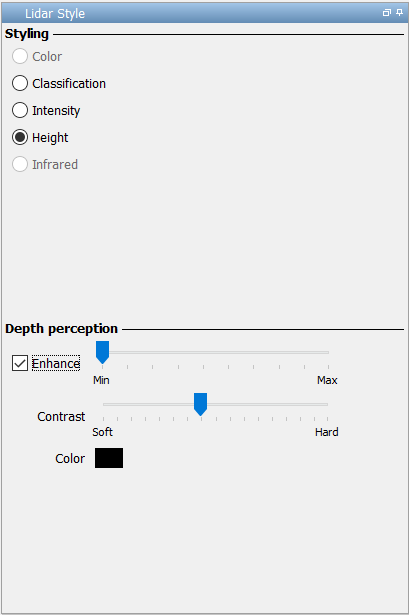
When the data is loaded, Lucy automatically selects a default styling for the points. To style the loaded data differently, use the options in the Lidar Style panel, as shown in Figure 19, “Selecting a LIDAR style”. Select the appropriate radio button to apply a particular styling based on the available information.
The selected option is applied to all LIDAR layers. If a certain layer does not support the styling, the layer is marked with a warning icon. If none of the layers support the styling, the corresponding radio button is grayed out.
The Lidar Style panel also provides options to enhance the depth perception of the point cloud data:
-
To improve the depth perception through an outline shading technique, select the Enhance check box. De-select the check box to disable the perception-enhancing techniques.
-
To increase the thickness of the applied shade, slide the upper Enhance slider to the right.
-
Use the Contrast slider to either soften or harden the applied shade.
-
To change the color of the applied shade, click the Color box to open a color chooser and select a new color.
Working with OGC GeoPackage, SQLite, SpatiaLite, and MBTiles data
Lucy allows you to work with a number of SQLite-based formats. You can:
-
Save and load vector and raster data from a GeoPackage file. GeoPackage is an OGC standard format based on SQLite. The OGC GeoPackage format is platform-independent, and suitable for use on mobile devices. You can load and save OGC GeoPackage files as .gpkg files.
-
Load vector data from an SQLite SpatiaLite file .
-
Save and load Luciad Vector DataBase (LVDB) and Luciad Raster DataBase (LRDB) files. The Luciad LVDB and LRDB formats are open SQLite file formats intended for the export of data. They offer functionality similar to the OGC GeoPackage format, with additional features such as styling.
-
Load data from MBTiles files. MBTiles is a file format for storing tiled data in SQLite databases. You can load MBTiles files with vector tiles or with image tiles in the JPG or PNG format.
Loading GeoPackage data and other SQLite-based formats
To visualize the contents of an SQLite-based format, go to File | Open… , select the appropriate file, and click OK.
You need to select a different file type for each of the SQLite-based formats:
-
OGC GeoPackage: Select a
.gpkgfile. A.gpkgfile can contain vector data as well as raster data. -
SpatiaLite: Select a
.splfile, which contains the properties of the vector data to load. -
LVDB and LRDB: Select either a
.lvdbor.lrdbfile. An.lvdbfile contains vector data. An.lrdbfile contains raster data. -
MBTiles: select am
.mbtilesfile that contains raster data or vector data.
Lucy will create a layer for the data you loaded. If you loaded an OGC GeoPackage file that contains both vector data and raster data, Lucy creates a layer tree with a sub-layer for each data type.
Saving GeoPackage data and other SQLite-based data
Lucy allows you to select either a vector layer or a raster layer, and save its contents to an SQLite-based file. You can save vector data to either OGC GeoPackage or LVDB files. Raster data can be saved to OGC GeoPackage or LRDB files.
Saving vector data
The vector data can originate from files like SHP, MIF and VPF files. Alternatively, you can create the data from within Lucy, with the drawing addon for instance.
Currently, you can save the following vector types:
-
Points
-
Polypoints
-
Polylines
-
Polygons
-
Complex Polygons
-
Shape lists that contain objects of the other types in this list
Other vector shapes will not be saved. Lucy displays an error message to notify you that it was not able to save an unsupported shape.
To save vector data:
-
Go to File | Save As…, and select the vector layer you want to save. The Save As… dialog box opens.
-
In the Files of type menu, select either
GeoPackage (*.gpkg)orLVDB (*.lvdb), depending on your preference. -
Indicate if you want to store all the data in the layer, or just the data currently visible on the map:
-
To store all data, select
Nonefrom the Cropping dropdown menu. -
To save just the data on the map, select the
Current Map Extentoption from the Cropping dropdown menu.
-
-
Click Save to save the vector layer.
Saving raster data
To save raster data:
-
Go to File | Save As…, and select the raster layer you want to save. The Save As… dialog box opens.
-
In the Files of type menu, select either
GeoPackage(*.gpkg) orLRDB(*.lrdb), depending on your preference. -
In the Compression format dropdown menu, indicate whether you want to compress the data to a JPEG file or a PNG file.
-
Use the Quality slider to set the quality of the image compression.
-
Indicate if you want to store all the data in the layer, or just the data currently visible on the map:
-
To store all data, select
Nonefrom the Cropping dropdown menu. -
To save just the data on the map, select the
Current Map Extentoption from the Cropping dropdown menu.
-
-
Select a Coordinate Reference System for your raster data from the CRS dropdown menu.
-
Click Save to save the raster layer.
Saving elevation data
To save elevation data:
-
Go to File | Save As…, and select the elevation layer you want to save. The Save As… dialog box opens.
-
In the Files of type menu, select
GeoPackage(*.gpkg). -
In the Elevation Compression format dropdown menu, indicate whether you want to compress the data to a PNG file or a TIFF file.
-
Use the Compression active checkbox to enable or disable compression.
-
Use the Quality slider to set the quality of the image compression.
-
Indicate if you want to store all the data in the layer, or just the data currently visible on the map:
-
To store all data, select
Nonefrom the Cropping dropdown menu. -
To save just the data on the map, select the
Current Map Extentoption from the Cropping dropdown menu.
-
-
Select a Coordinate Reference System for your elevation data from the CRS dropdown menu.
-
Click Save to save the elevation layer.
Loading the OBJ format
OBJ is a 3D file format developed by Alias WaveFront. You can load OBJ files in a 3D map using the File→ Open menu. Note that when opening an OBJ file you have to specify the georeference system as described in Specifying the georeference system.
Connecting to web service data
Instead of loading data onto your map from the file system, you can also connect to data offered by a web service. Make sure that the web service is up and running, before you try to connect to it.
To connect to web service data, go to File→ Connect To….
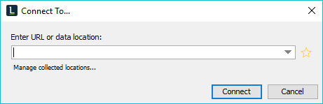
In the Connect To… dialog, enter the web service URL, and click Connect.
Lucy connects with the web service. To check the progress of the connection, see the Lucy status bar.
|
If you plan to connect to a particular data service often, it is recommended to mark it as a favorite. Click the Star icon next to the location URL box, and the web service will appear first in the location URL drop-down menu. To remove the data service as a favorite, select it from the drop-down menu, and click the Star icon again. |
Depending on the type of data service you are connecting to, Lucy may display an additional dialog box. That dialog box allows you to make further selections among the data offered by the service. For more information about these dialog boxes, see Working with the Fusion Client and Working with the OGC web clients for WMS, WMTS, WFS, and WCS services.
If Lucy cannot connect to the URL you provided, it will display an error message.
|
To connect to a 3D Tile service that serves 3D meshes or point cloud tilesets, specify an endpoint URL that ends in |
- Map-centric Lucy
-
To connect to web service data in map-centric Lucy, go to Data → Connect To…, or click the second icon in the top left corner of the application, Connect to web services using URLs….
Managing the collection of previous connections
Once you entered a new data URL and successfully connected with it, the URL will be stored for future usage. It becomes available in the location URL drop-down menu of the various client dialog boxes. Favorite data locations are listed first.
To remove URLs from the drop-down menu, click Manage collected locations/connections… below the drop-down menus. The Cache dialog box displays a list of previously entered URLs.
Your favorite data service URLs are marked with a filled Star icon. To remove a service as a favorite, click the Star icon in front of the data service location. You can also mark additional data sources as favorites by clicking the Star icon in front.
To remove a service URL, select it from the list, and click Remove selected. To clear all URLs from the locations list, click Remove all. If you want to remove all service URLs except your favorite ones, click Remove non-favorites.
Most Lucy connection clients come with a number of pre-defined service URLs in the locations collection. If you have accumulated a number of your own URLs in your collection of locations, you can remove all those extra URLs and keep just the pre-defined URLs by clicking Reset to defaults.
Working with the Fusion Client
The Fusion Client offers support for connecting to a LuciadFusion data service, and retrieving data from it. A LuciadFusion service serves data through the Luciad Tile Service (LTS) protocol.
Connecting the Fusion Client
To connect the Fusion client to a LuciadFusion service:
-
Select Map→ Data→ Fusion Client… to open the dialog box for the Fusion Client.
-
Enter the URL of a LuciadFusion data service or a LuciadFusion Tile Store in the LuciadFusion service URL box. The file URL for a LuciadFusion Tile Store must point to either a
tile-store.xmlfile or its parent directory.
Make sure that the LuciadFusion service is up and running, or that the LuciadFusion Tile Store directory exists, before you try to connect to it.
If you connected to a server before, you can select the URL of that server from the drop-down list. For more information about managing the URLs in that list, see Managing the collection of previous connections. -
Click the Connect button to connect to the URL as entered in the box. The box on the left displays the coverages served by the selected LuciadFusion service.
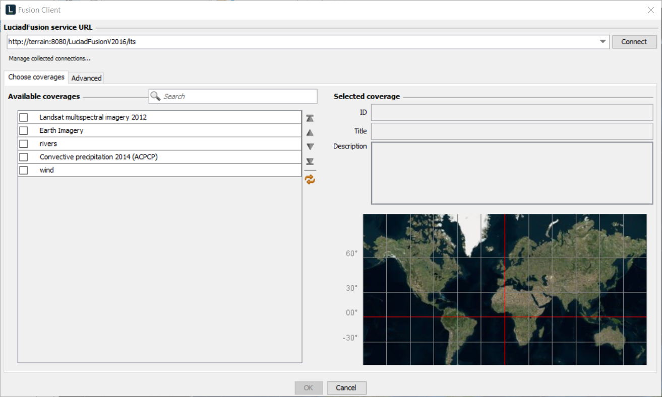
If the coverage list shows many coverages, you can find the one you need by entering a search term in the Search field.
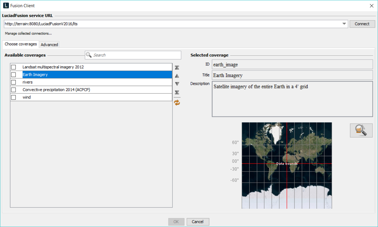
Click on a coverage to show its details in the panel at the right. If the coverage provides this information, you can see:
-
ID: the ID defined by the creator of the coverage.
-
Title: the current name of the coverage.
-
Description: a short description of the coverage.
-
A map preview of the geographic area covered by the coverage. To fit the map on the coverage, select the button at the top right of the map.
The Advanced tab displays a title and description for the service type you are working with.
On the map, for each selected coverage a corresponding layer is added.
Figure 22, “The Earth Imagery coverage retrieved in the Fusion Client” figure shows the Fusion Client dialog box with the retrieved coverages and the information for the Earth Imagery coverage.
Adding LuciadFusion coverages to the map
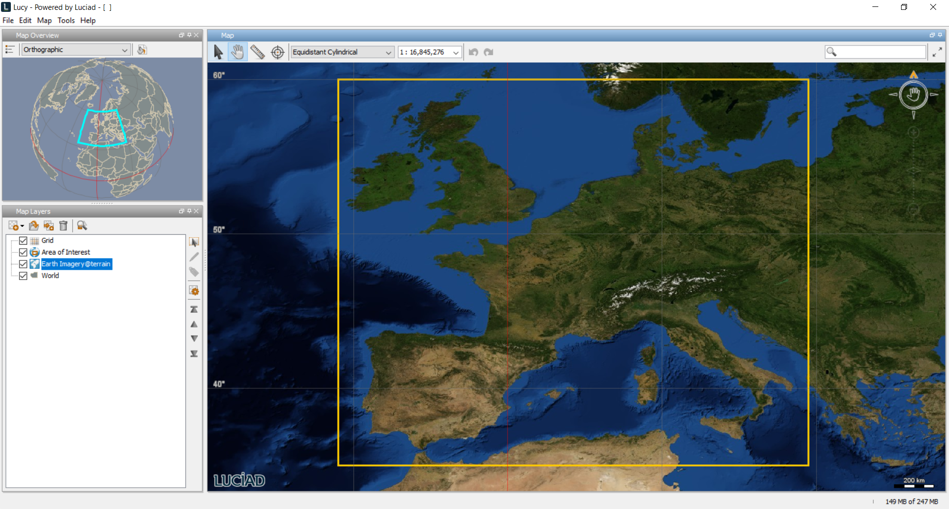
To create layers for the coverages, select the check boxes in front of the coverages and click OK. The layer is added to the Map Layers panel and the active layer is displayed in the Map panel as shown in Figure 23, “The Earth Imagery coverage displayed in Lucy GXY”. For more information on working with layers and visualizing layer data, refer to Working with layers.
- Map-centric Lucy
-
To connect to a LuciadFusion data service from map-centric Lucy, go to Data → Connect to…, enter the URL of the LuciadFusion service, and click Connect.
Working with the OGC web clients for WMS, WMTS, WFS, and WCS services
The OGC web clients offer support for connecting to and retrieving data from a number of web services that are compliant with the specifications and standards defined by the Open Geospatial Consortium (OGC). The supported web services are:
-
Web Map Service (WMS): for retrieving maps in the form of an image.
-
Web Map Tile Service (WMTS): for efficiently retrieving maps prepared as a tile structure.
-
Web Feature Service (WFS): for querying geographic data.
-
Web Coverage Service (WCS): for retrieving coverage data such as demographic information, weather charts, or elevation maps.
Connecting with an OGC web service explains how to set up an OGC service connection via the Lucy OGC clients. This setup is nearly identical for each of the supported web services. Retrieving and displaying WMS data, Retrieving and displaying WMTS data, Retrieving and displaying WFS data and Retrieving and displaying WCS data discuss the data selection and visualization specifics for WMS, WMTS, WFS and WCS respectively.
Connecting with an OGC web service
The connection to any OGC web service URL is always set up in the same way in Lucy.
You can select one of the available OGC web services from the Map→ Data menu. The connection dialog box for the selected web service opens.
Enter the URL of the OGC web service in the Service URL field, or select a URL from the dropdown menu, and click the Connect button. If you connected to a server before, you can select the URL of that server from the drop-down list. For more information about managing the URLs in that list, see Managing the collection of previous connections.
The dialog box displays the available layers on the Choose layers tab and the title and a description of the connected web service on the Service info tab.
If the client cannot connect to the URL you provided, it will display a Connection failed error message.
|
If you need to configure a web proxy, use Edit→ Proxy settings…. |
- Map-centric Lucy
-
To connect to an OGC web service from map-centric Lucy, go to Data → Connect to…, enter the URL of the OGC web service, and click Connect.
Retrieving and displaying WMS data
To connect the WMS client to a WMS:
-
Select Map→ Data→ WMS Client… to open the dialog box for the WMS Client.
-
Enter the URL of the service in the Web Map Service URL box.
-
Click the Connect button to connect to the URL as entered in the box. The box on the left displays the data served by the selected service.
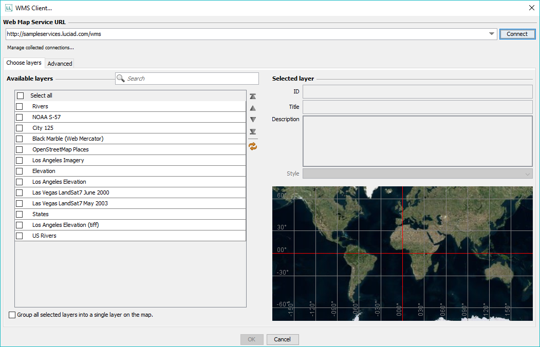
If the Available layers list shows many data sets, you can find the one you need by entering a search term in the Search field.
Click on a data set to show its details in the panel at the right. If the data set provides this information, you can see:
-
ID: the ID defined by the creator of the data set.
-
Title: the current name of the data set.
-
Description: a short description of the data set.
-
A map preview of the geographic area covered by the data set. To fit the map on the data set, select the button at the top right of the map.
Adding WMS data to the map
To display one or more available layers on the map, select the check boxes in front of the layers. To select all layers at once, select the Select all check box at the top of the layer list.
Click the OK button to add the selected images to the map. The layer tree contains a layer for each image and the images are displayed in the map view.
|
To group several selected WMS layers, and present the group as one layer on the Lucy map, select the Group all selected layers into a single layer on the map check box before clicking OK. You can control the order of the different layers in the group using the arrow icons next to the list. The benefit of grouping multiple layers into a single map layer is that Lucy needs to send less requests to the server. The drawback is that all data is grouped into a single map layer in Lucy, so you cannot control the order, visibility, … of individual layers. |
For more information about the style selection and server connection options, see Selecting a WMS layer style and Setting WMS service connection options .
Selecting a WMS layer style
WMS services may offer layer style definitions with the WMS layers. These determine which symbols and colors are used to display the WMS content.
To see what styles are available on the server for a particular layer, click the layer in the Available layers list, and open the Style drop-down menu. It will display the names of the available styles. Select one of the available styles to determine how the WMS layer will be displayed.
In many cases, only a default style will be available. If the layer definition on the WMS server does not contain any style element, the Style menu will display None. The WMS server determines how the WMS content is rendered.
Setting WMS service connection options
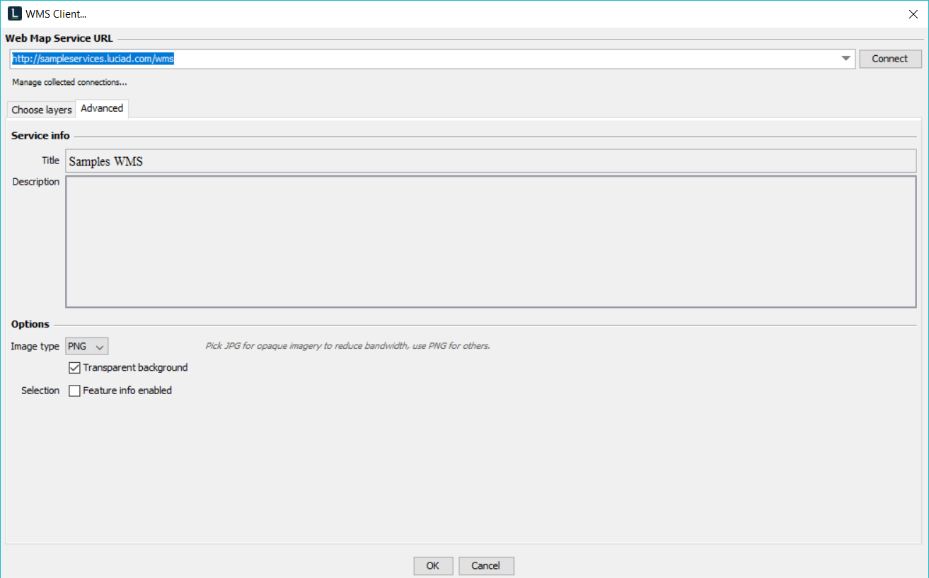
To select your server connection preferences, go to the Advanced tab. It displays the service title and description provided by the service, and an Options section:
-
The Image type drop-down menu shows the available file formats, and allows you to select your preferred file format for the retrieved image.
-
De-select the Transparent background check box if you prefer that the retrieved PNG image does not have a transparent background.
-
It is possible for Lucy users to select features from a WMS layer by clicking a certain location, and get more information about the selected features. To allow the service to send feature information when a user selects a WMS feature, select the Feature info enabled check box.
|
This functionality is dependent on technical prerequisites, such as the use of a select controller, and the creation of a
|
Modifying WMS data visualization
To change the layer’s properties, select the image layer from the layer tree and click on the Properties button in the layer toolbar or right-click the layer in the layer tree and select Properties from the menu.
You can:
-
Change the name of the layer.
-
Select a different paint style to display the layer in. You can choose between a Tiled and Non-tiled paint style. If you select Tiled, the requested WMS image will be returned as a collection of tiles, which offers a performance advantage: your image will be returned and visualized more quickly. To get a pixel-perfect image, without any potential artifacts, select Non-tiled.
Retrieving and displaying WMTS data
To connect the WMTS client to a WMTS:
-
Select Map→ Data→ WMTS Client… to open the dialog box for the WMTS Client.
-
Enter the URL of the service in the WMTS Service URL box.
-
Click the Connect button to connect to the URL as entered in the box. The box on the left displays the data served by the selected service.

If the Available layers list shows many data sets, you can find the one you need by entering a search term in the Search field.
Click on a data set to show its details in the panel at the right. If the data set provides this information, you can see:
-
ID: the ID defined by the creator of the data set.
-
Title: the current name of the data set.
-
Description: a short description of the data set.
-
A map preview of the geographic area covered by the data set. To fit the map on the data set, select the button at the top right of the map.
The Advanced tab displays a title and description for the service type you are working with.
On the map, for each selected coverage a corresponding layer is added.
Adding WMTS data to the map
To display one or more of the available layers, select the appropriate check boxes in the Available layers list. If the Style dropdown menu shows that more than one style is available for the selected layer, you can pick one of the styles.
Click the OK button to add the selected layers to the map. The layer tree contains a layer for each WMTS dataset.
|
In some rare cases, a |
Selecting a WMTS layer style
WMTS services may offer layer style definitions with the WMTS layers.
To see what styles are available on the server for a particular layer, click the layer in the Available layers list, and open the Style drop-down menu. It will display the names of the available styles. Select one of the available styles to determine how the WMTS layer will be displayed.
In many cases, only a default style will be available. If the layer definition on the WMTS server does not contain any style element, the Style menu will display None. The WMTS server determines how the WMTS content is rendered.
Modifying WMTS data visualization
To change the layer’s properties and styling, select the layer from the layer tree and click on the Properties button in the layer toolbar or right-click in the layer tree and select Properties from the menu.
Tips for optimal visual quality
-
WMTS layers have a number of fixed zoom levels. While Lucy will interpolate in between these levels, you will get the best visual results if you “snap” to a WMTS zoom level by using the mouse wheel on the map in combination with the CTRL key.
-
WMTS layers are defined in a fixed geographical reference. While Lucy will automatically "warp" the data to the current map projection, you will get the best visual results if you use the WMTS layer’s reference on the map. To do this, you can right-click on the layer in the layer control panel and select “Set layer reference to view”.
Retrieving and displaying WFS data
To connect the WFS client to a WFS:
-
Select Map→ Data→ WFS Client… to open the dialog box for the WFS Client.
-
Enter the URL of the service in the Web Feature Service URL box.
-
Click the Connect button to connect to the URL as entered in the box. The box on the left displays the data served by the selected service.
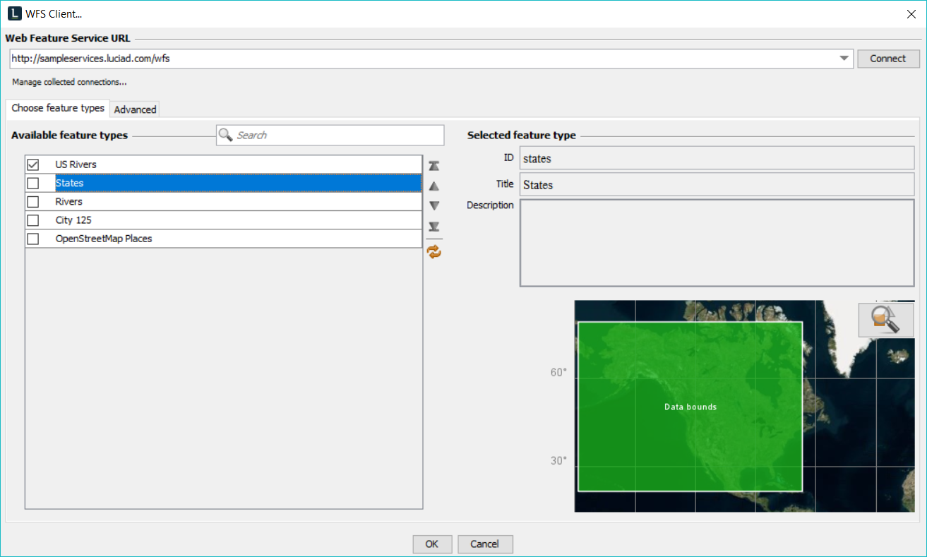
If the Available feature types list shows many data sets, you can find the one you need by entering a search term in the Search field.
Click on a data set to show its details in the panel at the right. If the data set provides this information, you can see:
-
ID: the ID defined by the creator of the data set.
-
Title: the current name of the data set.
-
Description: a short description of the data set.
-
A map preview of the geographic area covered by the data set. To fit the map on the data set, select the button at the top right of the map.
The Advanced tab displays a title and description for the service type you are working with.
On the map, for each selected coverage a corresponding layer is added.
Filtering requested features based on map area (Lucy GXY)
In Lucy GXY, you can use the Request features options on the Advanced tab to indicate how you want to filter the requested features:
-
To retrieve just the features in the visible map area, select that overlap with the view extent. Each time you zoom or pan on the map, the Lucy WFS client will request new features to match the visible map area.
-
To retrieve just the features in the Area of Interest, select that overlap with the area of interest. Each time you change the Area of Interest, the Lucy GXY WFS client will request new features to match the new AOI.
Adding WFS data to the map
To display one or more of the available feature types, select the appropriate check boxes in the Available feature types list. Click the OK button to add the selected feature types to the map. The layer tree contains a layer for each WFS data set.
Modifying the styling of the WFS data
To change the styling settings of the displayed data set, select the data set from the layer tree and click on the Properties button in the layer toolbar or right-click in the layer tree and select Properties from the menu. A dialog box allows you to select other styling settings for the features.
Retrieving and displaying WCS data
To connect the WCS client to a WCS:
-
Select Map→ Data→ WCS Client… to open the dialog box for the WCS Client.
-
Enter the URL of the service in the Web Coverage Service URL box.
-
Click the Connect button to connect to the URL as entered in the box. The box on the left displays the data served by the selected service.
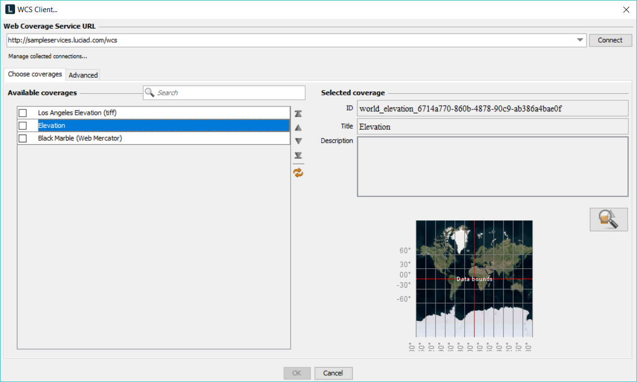
If the Available coverages list shows many data sets, you can find the one you need by entering a search term in the Search field.
Click on a data set to show its details in the panel at the right. If the data set provides this information, you can see:
-
ID: the ID defined by the creator of the data set.
-
Title: the current name of the data set.
-
Description: a short description of the data set.
-
A map preview of the geographic area covered by the data set. To fit the map on the data set, select the button at the top right of the map.
The Advanced tab displays a title and description for the service type you are working with.
On the map, for each selected coverage a corresponding layer is added.
Filtering requested features based on map area (Lucy GXY)
In Lucy GXY, you can use the Request features options on the Advanced tab to indicate how you want to filter the requested features:
-
To retrieve just the data for the visible map area, select that overlap with the view extent. Each time you zoom or pan on the map, the Lucy GXY WCS client will request new data to match the visible map area.
-
To retrieve just the data in the Area of Interest, select that overlap with the area of interest. Each time you change the Area of Interest, the Lucy GXY WCS client will request new data to match the new AOI.
Adding WCS data to the map
To display one or more of the available layers, select the appropriate check boxes in the Available coverages list.
Click the OK button to add the selected coverages to the map. The layer tree contains a layer for each WCS coverage.
Modifying the styling of the WCS data
To change the styling settings of the displayed data set, select the data set from the layer tree and click on the Properties button in the layer toolbar or right-click in the layer tree and select Properties from the menu. A dialog box allows you to select other styling settings for the coverage.
Connecting to Azure Maps
Azure Maps is a geospatial mapping service provided by Microsoft. It offers data such as worldwide road maps and high-resolution imagery. It replaces Bing Maps, which is deprecated and will be retired.
|
The first thing you need, before connecting to the Azure Maps servers, is an Azure Maps subscription key. The Azure Maps start page allows you to create an Azure account and an Azure Maps key. |
Licensing
You can request an Azure Maps subscription key from Microsoft by taking these steps:
-
Go to https://www.microsoft.com/en-us/maps/azure/get-started.
-
Click "Start for free".
-
Click "Try Azure for free".
-
Sign in with your Windows Live ID, or create one.
-
In the Azure Maps portal, click "Azure Maps Accounts". If you don’t see it, you can use the search field to find it.
-
Click on "Create".
-
Fill in the Instance details, such as name and region.
-
Click "Review + create".
-
In the account page, click "View authentication". This shows a primary and secondary key that can be used for Shared Key authentication.
-
Fill in the key when opening an Azure Maps layer in Lucy. See Using Azure Maps layers.
-
Alternatively, fill in the key in the file
config\lucy\azuremaps\TLcyAzureMapsAddOn.cfg
as the value of the
subscriptionKeyproperty.- Map-centric Lucy
-
To add the license key in map-centric Lucy, go to Data → Azure Maps → Edit Credentials….
You can obtain a license directly from Microsoft. Prices may vary according to the volume of licenses purchased, the duration of the license and the intended scope of use.
You can explore the pricing options at https://azure.microsoft.com/en-us/pricing/details/azure-maps/.
Using Azure Maps layers
Azure Maps imagery layers can be added in 2D and 3D views by selecting the _Map→ Data→ Azure Maps _ menu items. You can choose between imagery, roads, darkgrey roads, hybrid roads, hybrid darkgrey roads, road labels or darkgrey road labels.
- Map-centric Lucy
-
To add imagery layers in map-centric Lucy, go to Data → Azure Maps.
Tips
-
Azure Maps data has a number of fixed zoom levels. While Lucy interpolates in between these levels, you get the best visual results if you "snap" to an Azure Maps zoom level by using the mouse wheel on the map in combination with the CTRL key.
-
Azure Maps imagery is defined in a grid reference based on a Pseudo-Mercator projection and WGS 84 geodetic datum. Selecting the Pseudo-Mercator projection in the map toolbar avoids any overhead to "warp" imagery to another projection. Alternatively, you can right-click on the Azure Maps layer in the layer control panel and select "Set layer reference to view".
Connecting to Bing Maps
Bing Maps is a web mapping service provided by Microsoft, offering traditional road maps, aerial photo views, and searching capabilities. The Bing Maps imagery service is integrated by LuciadLightspeed.
|
Bing Maps is deprecated and will be retired by Microsoft. Only enterprise account customers can continue using Bing Maps for Enterprise services until June 30th, 2028. Free (Basic) account customers can no longer use Bing Maps and need to switch to Azure Maps. |
Licensing
If you are a Bing Maps enterprise account customer, you can request a Bing Maps license from https://www.bingmapsportal.com.
-
Fill in the created key when opening a Bing Maps imagery layer in Lucy (Using Bing Maps layers).
-
Alternatively, fill in the created key in the file
config\lucy\bingmaps\TLcyBingMapsAddOn.cfg
as the value of the application ID property.
- Map-centric Lucy
-
To add the license key in map-centric Lucy, go to Data → Bing Maps → Edit Credentials….
Using Bing Maps layers
Bing Maps imagery layers can be added in 2D and 3D views by selecting the _Map→ Data→ Bing Maps _ menu items. You can choose between roads, aerial imagery, labeled aerial imagery, a dark canvas, a light canvas, or a gray canvas base map.
- Map-centric Lucy
-
To add imagery layers in map-centric Lucy, go to Data → Bing Maps.
You can also add custom layers from data providers offering Bing Maps compatible imagery. The URI pattern should contain a \ wild card. The wild card will be replaced with unique tile identifiers to allow retrieving the necessary imagery. To open a custom Bing Maps URL, select Map→ Data→ Custom Bing Maps… or File→ Connect To….
Refer to the Microsoft Developer Network http://msdn.microsoft.com/ for more information on the Bing Maps URL pattern and the Bing Maps tiling structure.
Tips
-
Bing Maps imagery has a number of fixed zoom levels. While Lucy will interpolate in between these levels, you will get the best visual results if you "snap" to a Bing Maps zoom level by using the mouse wheel on the map in combination with the CTRL key.
-
Bing Maps imagery is defined in a grid reference based on a Pseudo-Mercator projection and WGS 84 geodetic datum. Selecting the Pseudo-Mercator projection in the map toolbar will avoid any overhead to "warp" imagery to another projection. Alternatively, you can right-click on the Bing Maps layer in the layer control panel and select "Set layer reference to view".
Consulting warning and error logs
You can encounter warnings or errors when you load data or try to connect with a data service. The data set is only partially loaded, for instance, or the data format is not supported out of the box. If such a warning or an error is logged, Lucy displays it in the status bar. If multiple errors have been logged, you can click a link in the status bar to open an error and warning messages panel.
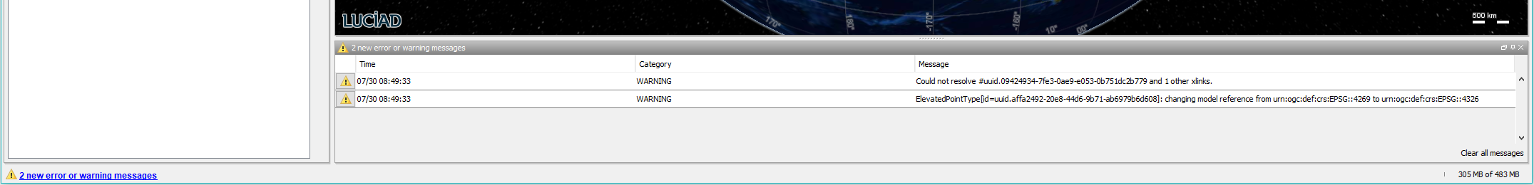
To review all logged warnings and errors from the menu, go to Tools → Show error log. The warning and error messages panel opens, and lists all previously logged messages. Click Clear all messages in the lower right corner of the panel to remove all the messages logged so far from the list.
- Map-centric Lucy
-
If any warnings or errors occur during data loading, for example, map-centric Lucy notifies you. It shows you error messages and pop-ups. The bottom icon in the side tool bar changes to:
-
 Lucy has registered an error message. Click the icon to view the error in a list of warning and error messages.
-
 Lucy has registered a warning message. Click the icon to view the warning in a list of warning and error messages.
Double-click the warning or error in the list to view the message details in a pop-up box. If you have finished revising the list of messages, you can delete them from the message view by clicking Clear all messages.
Loading and saving workspaces
You can customize Lucy’s user interface to your preferences and needs by loading map data of your choice, rearranging the different panels, and opening different maps. Lucy’s workspace concept allows you to save customized user interfaces for different sessions and users.
Workspaces are stored in .lws format and contain the settings of the current user interface but not the loaded data files. A snapshot of the Lucy map view is stored alongside the workspace file when you save it for the first time. This makes it easier to find and open the workspace again. The snapshot will be shown in the Lucy file chooser when you select the workspace file in it.
You can store the data files in any location but the recommendation is to store them in the same folder as the workspace file or in a subfolder. The workspace file will then contain references to the data files using relative paths instead of absolute paths. This is useful if you want to copy the workspace together with the data files to another location or if you want to open the workspace from another computer.
Lucy loads a workspace on startup. To save changes to that workspace in another workspace file, use the File→ Save Workspace As menu item. A dialog box appears that allows you to name the new workspace file and save it to the default workspace folder or to another location.
Use the File→ Open Workspace or File→ Open menu item to open a workspace and load its data files. Note that you can only open one workspace at a time. To make finding the right workspace within a collection of files easier, the Lucy file chooser shows a thumbnail image of a workspace when you select it.
To overwrite the settings of the loaded workspace with the current workspace settings, use the File→ Save Workspace menu item.
To make the current workspace the workspace that is loaded on startup, select the File→ Set startup workspace menu item. The workspace will then be loaded when starting Lucy. To undo this action and make the original workspace the one that is loaded on startup again, select the File→ Set startup workspace menu item and click on the Restore original button in the dialog box that pops up.
- Map-centric Lucy
-
To open a workspace in map-centric Lucy, go to menu{Data→ Open…}, and select a workspace file. To save changes to a workspace in a workspace, go to Data→ Save Workspace. To save changes to a workspace in a different workspace file in map-centric Lucy, go to Data→ Save Workspace As….
Working with layers
The map as shown in the map view is the visualization of one or more layers, each containing a set of geographic data. This section describes the layer tree, the layer tools, and the layer properties and their relation to the map view. Loading and saving map data provides more information on loading and saving map data.
The layer tree
The layer tree in the Map Layers panel shows the separate layers of the map and has a similar function as the legend on a paper map. The check box next to the layer indicates if the layer is visible on the map or not. The icon next to the layer name shows the painting style that is used to represent the layer in the map view. Grouped layers have a plus icon next to them; click on the plus icon to expand the list and click on the minus icon to collapse an expanded list. Figure 30, “A Map Layers panel with an expanded AIXM 5.1 layer” shows the Map Layers panel with an AIXM 5.1 layer expanded in the layer tree.
|
The busy icon |
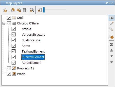
The layer tools and options describes the icons in the toolbar above the layer tree.
The layer tools and options
The toolbar in the Map Layers panel offers tools to perform actions with the map layers. You can only use these tools if one or more layers are selected. To select a layer, click on the layer in the layer tree. To select multiple layers, keep the Ctrl-key pressed while clicking on the layers. The selected layers are highlighted as shown in Figure 30, “A Map Layers panel with an expanded AIXM 5.1 layer”.
The following layer tools are available:
-
 The Add layer icon. With this icon you can add a layer for drawing shapes on the map as described in Drawing shapes on the map.
-
 The Open icon. When pressing this icon, a dialog box pops up allowing you to select files from which to load data.
-
The Copy layers from another map icon. With this icon you can copy one or more layers from another map as described in Copying layers from another map.
-
 The Delete icon removes the selected layer(s) from the map.
-
 The Fit to layer icon fits the map view to the (union of the) selected layer(s).
-
 The Change layer transparency slider lets you adjust the transparency of the layer. Slide it to the right to increase the transparency of the selected
layer. If you cannot see the icon, click the
The Change layer transparency slider lets you adjust the transparency of the layer. Slide it to the right to increase the transparency of the selected
layer. If you cannot see the icon, click the  icon, or expand the Map Layers panel to the right.
-
 The Layer Selectable icon makes the selected layer(s) selectable which means that you can select objects from the layer(s) in the map view with
the Select tool as described in The map tools.
The Layer Selectable icon makes the selected layer(s) selectable which means that you can select objects from the layer(s) in the map view with
the Select tool as described in The map tools.
-
 The Layer Editable icon makes the selected layer(s) editable which means that you can edit objects from the layer(s) in the map view with the
Select tool as described in The map tools. Editing data provides more information on editing data.
The Layer Editable icon makes the selected layer(s) editable which means that you can edit objects from the layer(s) in the map view with the
Select tool as described in The map tools. Editing data provides more information on editing data.
-
 The Layer Labeled icon adds labels to the objects of the selected layer(s) in the map view. Note that if many labels are added or if labels
are too big, the labels might overlap each other. To prevent labels from overlapping, select the Map→ Global label decluttering menu item as described in Enabling global label decluttering (Lucy GXY). Note that this setting applies to all labels on the map, not only the labels of the selected layer(s).
The Layer Labeled icon adds labels to the objects of the selected layer(s) in the map view. Note that if many labels are added or if labels
are too big, the labels might overlap each other. To prevent labels from overlapping, select the Map→ Global label decluttering menu item as described in Enabling global label decluttering (Lucy GXY). Note that this setting applies to all labels on the map, not only the labels of the selected layer(s).
-
 The Layer Properties icon shows a panel with the properties of the selected layer as described in The layer properties panel. If multiple layers are selected, the properties panel shows the properties that the selected layers have in common.
The order of the layers in the tree reflects the order in which the layers are rendered in the map view. To change the order of the layers use the following icons which are located next to the tree:
-
 The Move Selected Layers to Top icon moves the selected layer(s) to the top of the layers tree.
-
 The Move Selected Layers Up icon moves the selected layer(s) one level up in the layers tree.
-
 The Move Selected Layers Down icon moves the selected layer(s) one level down in the layers tree.
-
 The Move Selected Layers to Bottom icon moves the selected layer(s) to the bottom of the layers tree.
When you right-click in the layer tree, a menu pops up with all the layer tools and the following additional layer options:
-
The Scale to raster level option (Lucy GXY) only applies to raster layers and is enabled if only one raster layer is selected. This option scales the map so that it visualizes the raster pixels one-on-one to the screen pixels. If the raster has multiple levels, a dialog pops up in which you can select the preferred level. The raster scale as described in Using the raster scale (Lucy GXY) provides the same functionality.
-
The Set layer reference to view option sets the projection of the map view to the reference system of the layer source. This option is enabled if only one layer is selected. Using this option improves the rendering performance of the selected layer because it avoids projection calculations. This option is useful for raster layers.
-
The Table View option opens a separate panel under the map view for each selected layer. The table view shows the layer’s objects and their properties in table format. Displaying your data in a table view describes the table view in more detail.
-
The Visible option allows you to display or hide a layer in the map view. This option controls the check boxes next to the selected layers in the list.
-
The Snap to layer option (Lucy GXY) sets snapping on or off for objects in the selected layer(s). While editing an object such as a path it may be convenient to snap to the (corner) points of an existing object on the map such as a harbor or a boat. Select the Snap to layer option for the layer that contains the objects that you want to snap to. Turn snapping off for a layer that contains objects that you do not want to snap to while editing, such as the world layer.
The layer properties panel
Each layer has a set of properties that you can view and change in the layer properties panel. To open the panel for one or more selected layers, right-click in the layer tree or click on the Layer Properties icon in the toolbar. If multiple layers are selected, the panel will only show the properties that the layers have in common. As the properties of a layer depend on the data type of the layer, the properties panel might be different for the different layer types.
The layer properties panel contains the following tabs:
-
General --- This tab shows the general layer properties such as the source, label (or name), and the settings as defined by the layer tools and the layer options in the pop-up menu. You can change the styling of Lightspeed layers by sliding the Transparency, Contrast and Brightness sliders to the required setting.
-
Paint style --- This tab shows the properties of the paint style that is used to represent the layer in the map view. The properties in this tab can differ depending on the layer type. The layer paint style describes the layer paint style in more detail.
-
Label style --- This tab shows the properties that are used for the labels of the layer. If the layer has no labels, this tab will not be shown. Figure 31, “The Label style tab of the world layer” shows the Label style tab of the world shape layer. Double-click the font name to open a font selector dialog box in which you can change the font settings. Double-click the color boxes to open a color selector dialog box in which you can change the colors as described in The color selector. You can also add a halo around the labels and specify its color and thickness.
-
Band selection --- This tab shows band selection options for multi-spectral imagery. Multi-spectral images consist of data captured on multiple, possibly invisible bands of the geomagnetic spectrum, such as infrared bands. To derive useful information from such images, you can select three bands in a specific combination, and map them to the RGB color channels. For more information, see Layer band selection.
After changing the settings, click on Apply to display the layer in the map view with the new settings. To accept the new settings, click on OK, otherwise click on Cancel.
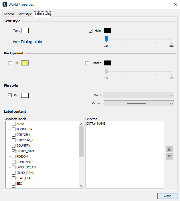
The layer paint style
|
If you style your layers with SLD, you can configure a much more complex styling for your layers. Simply store the |
The paint style that is used to represent the layer in the map view depends on the data type of the layer. Figure 32, “The Paint style tab of a layer with vector data” shows the Paint style tab of a vector data layer.
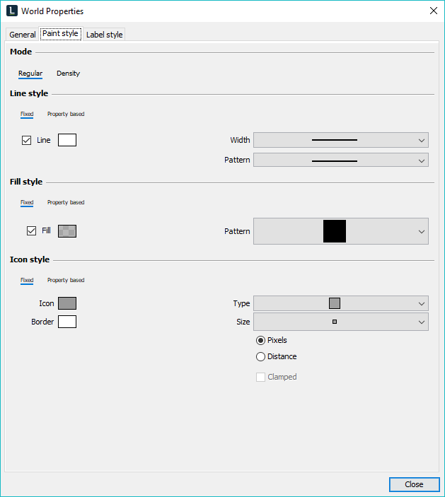
The Paint style tab of a vector layer allows you to set a regular paint style or a density paint style.
Regular vector layer styling
Within the regular paint style options in Lucy, you can choose to style all the objects in your layer identically, or let the properties of the data in your layer determine what they look like.
To style the lines, fills or icons of all the objects in your layer identically, select the Fixed option in the Line style, Fill style or Icon style sections. The fixed regular paint style allows you to select the line width, the line color, and the fill color and pattern of the layer data, as well as the styling of any icons in the layer. To pick different colors, click the color rectangles and open a color selector dialog box in which you can change the colors as described in The color selector.
To differentiate the styling of layer objects based on the values of object properties, select the Property based option in in the Line style, Fill style, or Icon style sections.
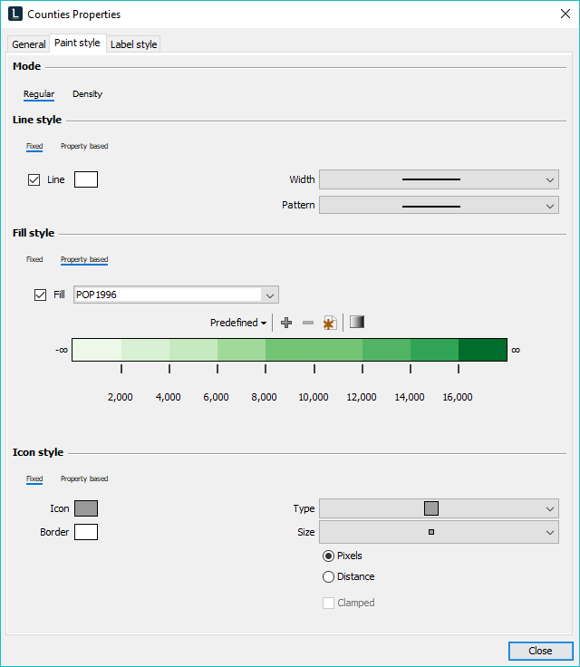
You can apply property-based styling if the objects in your layer have a color property or at least one property with numerical values, such as a population count number for a city object.
Color properties are automatically matched to the right colors.
|
It is possible to mix styling options, and select a fixed style for one shape component, and a property-based style for another shape component. For instance, you can choose a fixed line style to make all the country borders look the same, while you fill the country shapes with distinct colors based on the population property of the country. |
To map the value range of a property to a color map, first select the property from the drop-down menu. Then select a pre-defined color mapping from the pre-defined dropdown menu. The color mapping is completely customizable. You can change:
-
The start value of the property-to-color mapping, the end value of the property-to-color mapping, and the delta value that determines at which point there is a transition to the next color in the range.
-
The colors in the color map and the transition points between the colors
-
Whether the colors transition abruptly, or in a gradient.
For more information about using the color map tools to change the color map, see The color bar.
Density layer styling
The Density style for vector data paints layer data according to the number of objects present in a particular area on the map. Layer areas containing a high number of objects are colored differently from areas with lower object numbers. This kind of representation is often called a density plot or heat map.
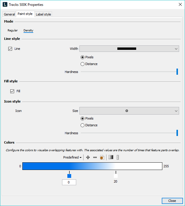
You can specify how you want your density plot to look with the Density layer properties:
-
You can determine the width of lines in your density plot, and choose whether the width is specified in screen Pixels or world Distance. A density plot with pixel-sized width adapts when the zoom level changes. With world-sized density, the width is specified in distance, with respect to the world reference. A density plot with world-sized width remains fixed when the zoom level changes. An example of world-sized data is a data set of roads, in which the road widths are specified in world sizes, 8 meters for instance.
-
Similarly, you can choose whether the size of the icons in your density plot is specified in pixels or in distance. The Fill check box allows you to determine whether polygons in your density plot are filled or not.
-
You can change the color range in which the density plot is displayed. The Predefined drop-down menu allows you to choose from a number of predefined color ranges. In addition, you can use the color bar to change or further refine the color variation in your density plot. See The color bar for more information.
Styling point clouds
If you connect to an OGC 3D Tiles service to visualize a point cloud layer, you also have access to a styling tab in the layer properties panel. The color properties in the point cloud are applied automatically. You can choose to map other point cloud properties to a color map of your choosing. You can also change the shape and size of the icons representing the points in your point cloud.
|
3D point cloud tilesets are typically the result of tiling and multi-leveling large amounts of LAS and LAZ (LASZip) data for improved loading and visualizing performance. You can also load individual LAS and LAZ files in Lucy. For more information, see Loading LIDAR data. |
Lucy can visualize distinct properties of the points in the point cloud,such as:
-
Color: uses the color information available in the data.
-
Height: shows the height of a point as a color in gradient color range mapped to a height range.
-
Classification: shows a different color per class.
-
Intensity: shows the intensity reading available in the data as a color in a color range.
The color mapping styling options depend on the information available in the tileset. Other available information may be infrared readings, or laser return numbers.
To select styling options, open the layer properties panel, and go to the Icon style tab.
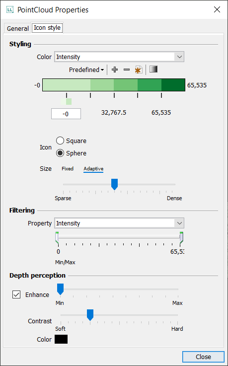
Icon styling
To map a point property to a color range:
-
In the Color drop-down menu, select the information type you want to use to style the point data with.
The icon Color information is applied straightaway as the default point styling, and does not require any mapping to a color range.
-
To map the value range of another point cloud property to a color map, first select the property from the drop-down menu. Then select a pre-defined color mapping from the Predefined drop-down menu. The color mapping is customizable. You can set or change:
-
The start value of the property-to-color mapping, the end value of the property-to-color mapping, and the delta value that determines at which point there is a transition to the next color in the range.
-
The colors in the color map and the transition points between the colors
-
Whether the colors transition abruptly, or in a gradient.
For more information about using the color map tools to change the color map, see The color bar.
By default, the individual points are represented as spheres. You can switch the spheres to Square shapes in the Icon section of the Icon style tab.
You can also control the size of your icons. If you want the icons to have a constant size, regardless of the density of the point cloud, select the Fixed option in the Size section. Drag the slider to select a pixel size for your icon.
If you want the size of the point icon to adapt to the local density of the point cloud, select the Adaptive option. As a result, the point cloud layer becomes more visually continuous and opaque. You can still adjust the density level to more sparse or more dense by dragging the slider below to the left or the right.
Filtering
Lucy allows you to focus on a specific value range of a point property, and remove the points outside that range from the visualization. To show only the points that fall within a specific range:
-
Go to the Filtering section of the Icon style tab.
-
Select the point property that you want to filter from the Property drop-down menu. The slider below shows the available value range for that property.
-
Drag the slider handles to new positions to narrow the range of visualized points. The points outside the range disappear from the map.
To narrow the value range you are working with, click the Min/Max button below the slider. If you specify a higher minimum value, and a lower maximum value in the Min/Max dialog, the points falling outside that range are filtered out already, and you are left with a smaller working set on the map.
Improving depth perception
Finally, you can further manipulate the perception of depth in the visualized point cloud through an outline shading technique.
To improve the depth perception:
-
Go to the Depth perception section of the Icon style tab.
-
Make sure that the Enhance check box is selected.
-
To increase the thickness of the applied shade, slide the upper Enhance slider to the right.
-
Use the Contrast slider to either soften or harden the applied shade.
-
To change the color of the applied shade, click the Color box to open a color chooser and select a new color.
-
Raster data styling
Figure 36, “The Paint style tab of layer with raster data” shows the Paint style tab of a GeoTIFF image, containing raster data.
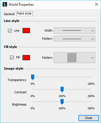
The Paint style tab in Lucy GXY contains some specific settings that are applicable to images.
|
For raster layers, the recommendation is to keep the default settings and only change them for exceptional use cases. |
-
Paint outline --- This option indicates if an image outline is shown or not in case the number of raster pixels per screen pixel is higher than the Start resolution factor (see below).
-
Outline color --- The color of the image outline.
-
Force painting --- Indicates if an image should be displayed or not irrespective of the used scales (see below). When this option is enabled, loading of large amounts of data is possible so it is best to only select this option for exceptional use cases and deselect this option after use.
-
Level switch factor --- This setting is only available for multi-leveled raster data and determines the scale point at which a raster level is selected. The default value is 1 which means that as soon as a single raster pixel would be displayed by multiple screen pixels, a higher resolution level of the image is selected to display the image. If the level switch factor is smaller than 1, the image may become pixelated but it can optimize the rendering performance.
The view scales for which the raster should be visible can be customized in the Scale ranges tab, as shown in figure Figure 37, “The Raster scales tab of a layer with raster data”. This tabs allows you to manually specify between which view scale levels the raster should be shown, and for which scales the raster should be hidden. The arrow icons allows to revert back to the original values.
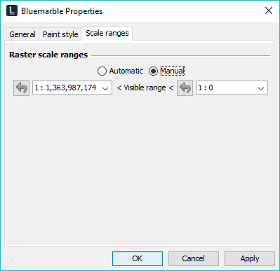
Note that it is possible to save the current settings of the layer properties by saving the current workspace. The next time that the workspace is opened, the layer will have the settings as defined when saving the workspace. It is also possible to save the layer properties to a style file which can be loaded every time the data is loaded, irrespective of the workspace settings. The layer style file describes the layer style file in more detail.
The layer style file
To keep all the changes that are made to the layer properties and use the same properties every time the layer is loaded, it is possible to save the layer settings to a layer style file. The layer style file stores the current properties of the layer separate from the layer data file.
To save the changed properties of a layer to a style file either choose:
-
File→ Save Layer Style --- This option allows you to save the properties of a selected layer to a layer style file in the same location as the layer data file. Use this option if the style file should always be loaded together with the data file.
-
File→ Save Layer Style As --- This option allows you to save the layer properties to a layer style file in another location as the layer data file. Use this option to save different style files for different configurations.
|
Note that the style file will only be opened when the data file is loaded. When opening a workspace, the style settings as saved with the workspace are restored. To open the style file make sure to load the data file by using the File→ Open menu item or by dragging and dropping it from your file system. |
Layer band selection
Remote sensing imagery, such as the images captured by satellite sensor equipment, consists of multiple spectral bands. They each capture sensor information on one band of the geomagnetic spectrum. For instance, Landsat 7 images consist of the bands blue, green, red, near infrared (NIR), Shortwave Infrared (SWIR) 1, thermal, SWIR 2, and panchromatic.
To visualize and analyze the information captured on invisible bands, Lucy allows you to map the bands to the Red, Green, and Blue color channels. You can set up your own mapping, or use one of the preset mappings made available by Lucy.
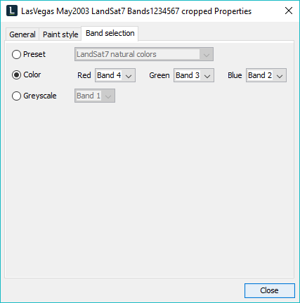
-
Presets Select pre-defined band combinations that each provide a different perspective on the image captured. For example, one of the presets is Landsat7 near infrared. That band combination is applicable to images captured by the Landsat 7 satellite, and highlights information captured on the near infrared band. Near infrared data is suitable for the detection of vegetation. You can select your own band combination presets in the
TLcyLspLayerCustomizerAddon.cfgconfiguration file. -
Color Define your own band combination and select the bands you want to map to the Red, Green or Blue color channel.
-
Greyscale Select just one band of the image, and display it as a grayscale image.
Working with multiple maps
You can add a new map by using the File→ New→ Map menu item. The map view shows the tabs of the maps that are opened. Click on the tab of a map to make that map active. When a map is active, the menu items and settings only apply to that map. The Map view and Map Layers panel display the active map and layers.
|
When multiple maps display the same data you can synchronize the view of all maps to the selection of data in the active map by selecting the Map→ Synchronize selection menu item. |
Copying layers from another map
To copy one or more layers from another map to the active map, click on the Copy layers from another map icon![]() in the layer control toolbar. A dialog box appears as shown in Figure 39, “The dialog box for copying layers from one map to another”. If multiple maps are open, select a map from the drop-down list. The layer tree shows the layers of the selected map. Select
the layer in the layer tree by clicking on the layer. To select multiple layers, Shift- or Ctrl-click on the layers in the
layer tree. Click on OK to copy the selected layers to the active map or click Cancel to close the dialog box without copying
layers.
in the layer control toolbar. A dialog box appears as shown in Figure 39, “The dialog box for copying layers from one map to another”. If multiple maps are open, select a map from the drop-down list. The layer tree shows the layers of the selected map. Select
the layer in the layer tree by clicking on the layer. To select multiple layers, Shift- or Ctrl-click on the layers in the
layer tree. Click on OK to copy the selected layers to the active map or click Cancel to close the dialog box without copying
layers.
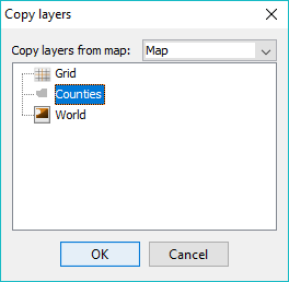
|
When you copy layers from one map type (2D or 3D) to another and the file format is not supported in the target map, the status bar shows a message that the layer could not be transferred. |
Working with dynamic data
Lucy provides tools to work with dynamic data, such as data with a time component and moving objects.
Using the Previewer
|
Before loading dynamic data, make sure that the component that supports your dynamic data set is installed, such as the Aviation Standards or Radar Connectors components. |
The Tools menu displays a Previewer menu item. When you select this item, the Previewer panel appears in the top left corner of the application window. Figure 40, “The Previewer panel” shows an example of the Previewer panel.
The Previewer panel allows you to visualize and control the progress in time of dynamic data on the map.
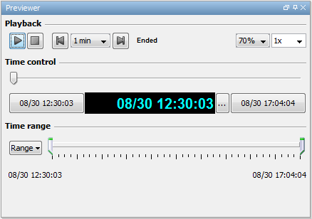
The Playback section provides the following functionality:
-
 Start the playback. When the playback is started, the icon changes into the Pause icon.
-
 Pause the playback. When the playback is paused, the icon changes into the Start icon.
-
 Stop the playback. When the playback is stopped, the current Previewer time is reset to the start time of the selected data
set.
Stop the playback. When the playback is stopped, the current Previewer time is reset to the start time of the selected data
set.
-
 Skip backward in the playback. You can only select this option if the playback is not active. The time to skip is indicated
in the box at the right right of the icon. To skip the simulation repeatedly, keep pressing the icon.
Skip backward in the playback. You can only select this option if the playback is not active. The time to skip is indicated
in the box at the right right of the icon. To skip the simulation repeatedly, keep pressing the icon.
-
 Skip forward in the playback. You can only select this option if the playback is not active. The time to skip is indicated
in the box at the left of the icon. To skip the simulation repeatedly, keep pressing the icon.
Skip forward in the playback. You can only select this option if the playback is not active. The time to skip is indicated
in the box at the left of the icon. To skip the simulation repeatedly, keep pressing the icon.
The first of the list boxes on the right in the Playback section controls the maximum CPU usage that the previewer can consume. The second list box controls the relative speed of the playback. Click in the drop-down list to select other values.
Use the Time control slider to manually control the playback time. The three boxes below the slider show the start time, the current Previewer
time, and the end time of the playback. To specify a different Previewer time, click on the icon next to the current time
![]() to open a calendar selection box and select a time.
to open a calendar selection box and select a time.
The sliders in the Time range section control the playback time, as shown in the Time control section. The full time range is the union of the time ranges of all data sets. Adjusting the time range allows you to focus on a smaller time frame.
You can also set the time range of the playback to the time range of one particular data set by:
-
Selecting that data set in the Range list box.
-
Right-clicking the required data set in the Map Layers panel, and select Use time range from the pop-up menu.
-
Right-clicking on a map object, and select Use time range from the pop-up menu.
The time ranges in the Time control and Time range sections are adjusted to the time setting of the data.
To reset to the full time range, use the Reset item in the Range list box, or double-click the sliders.
|
If you are displaying the same data set simultaneously in a 2D map and a 3D map, you only need one previewer to control data playback in both maps. If you start the playback, for example, the playback will start running on both the 2D and the 3D map. |
- Map-centric Lucy
-
If you load dynamic data with a time aspect, map-centric Lucy automatically displays previewer controls on top of the map.
Linking a camera to a moving object
You can link a camera to an object moving on the map, to follow the object from the perspective of the camera.
On a 3D map, activate the camera view by right-clicking on a selected object and choosing the Follow Object menu item. You can then select one of the following camera options:
-
Look from selected object(s): The camera is linked to the object and looks from the object while it moves. Note that by moving the mouse you can change the viewing direction of the camera.
-
Look at selected object(s): The camera looks at the object while it moves and follows the movements of the object, for example when it changes direction. Note that you can change the viewing direction and the position of the camera by moving the mouse.
On a 2D map in Lucy GXY, select the object in the map, right-click and select the Link menu item. When multiple maps are opened, select This map. You have the following camera options:
-
Don’t link: the camera is not linked to the selected object. When the object follows a track, the object moves but the map and compass grid (if enabled) do not move. This option is selected by default.
-
Center selected object: the camera is linked to the selected object and when the object follows a track, the object and compass grid (if enabled) are re-centered in the map. The map view changes to keep the object in the center of it.
-
Follow selected object: the camera is linked to the selected object and when the object follows a track, the map rotates with the direction of the object and the compass grid (if enabled) follows the object.
To deactivate the camera select the menu option Don’t link.
Editing data
This article describes how to edit object properties, copy and paste objects, change the measurement settings and colors, and how to undo and redo changes.
Editing object properties
When an object is selected on the map it is possible to view and change the properties of the object in a separate panel. To open the Object properties panel for a selected object, either right-click on the map and select Properties from the menu that appears or select the Map→ Object Properties menu item. The Object properties panel only shows the properties of one selected object. The contents of the Object properties panel changes when selecting another object. When multiple objects are selected, no object properties are shown.
Drawing shapes on the map describes the properties for the different shapes. You can find more examples of the Object properties panel throughout this guide. Figure 41, “The Area of Interest properties panel for Europe” shows an Area of Interest properties panel, which is an object properties panel specific to Areas of Interest, as described in Defining an Area of Interest (Lucy GXY)).
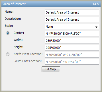
Some Object properties panel display property hierarchies, such as the properties panels for AIXM objects. See Figure 76, “The comparison view of two AIXM objects located below the map view” for examples of those panels. These hierarchical property panels open with the hierarchical properties collapsed below the top hierarchy level. You can display the full hierarchies by expanding one of the collapsed properties, or by clicking the Expand all icon at the top of the panel. Unspecified read-only object properties are also hidden by default. Click the Filter icon to display these properties.
Copying and pasting objects
Note that the copy functionality only works on a limited set of vector data and the paste functionality only works on editable layers. It is possible to paste objects to the same or to a different layer. Perform the following steps to copy (or cut) and paste objects from one layer to another:
-
Select the object(s) on the map as described in The map tools.
-
Select the Edit→ Copy menu item (or press Ctrl+C) to copy the object(s) from the layer, or; select the Edit→ Cut menu item (or press Ctrl+X) to cut the object(s) from the layer.
-
Go to the layer tree and select the layer to which you want to paste the object(s).
-
Select the Edit→ Paste menu item (or press Ctrl+V).
Note that a pasted object will adapt to the settings of the layer to which it has been pasted and thus it may appear differently than in the originating layer. This can, for example, apply to the display color of the object.
Setting units, formats, and the coordinate system
To change the measurement unit to display distance, altitude, and speed for all data, use the following menu items respectively:
-
Edit→ Distance unit, options are: Meter, Kilometer, Nautical Mile, Mile US, and Feet
-
Edit→ Altitude unit, options are: Meter, Kilometer, Flight Level, and Feet
-
Edit→ Speed unit, options are: Meter/Second, Kilometer/Hour, and Knots
To change the format for displaying angles, date and time, duration, and coordinates use the following menu items respectively:
-
Edit→ Angle Format
-
Edit→ Date Time Format
-
Edit→ Duration Format
-
Edit→ Point Format: allows you to change the format of the latitude-longitude coordinates. Options are: Georef, Lat Lon, MGRS (requires the Defense Symbology component), and BNG.
|
Note that the settings described in this section apply to all GUI elements of the Lucy application. |
Specifying the coordinate system
To display data, Lucy offers the possibility to either use:
-
The original coordinate system. This means that the data is displayed in the coordinate system of the data source. Data from multiple sources with different coordinate systems will thus be displayed in different coordinate systems. This is the default setting. When a custom coordinate setting is defined, you can switch to the original coordinate system by selecting Edit→ Coordinate System→ Original Data Coordinate System.
-
A custom coordinate system. This means that all data is displayed in one predefined or custom coordinate system. You can choose or define a custom coordinate system by selecting Edit→ Coordinate System→ Choose coordinate system. A dialog box appears in which you can choose between two coordinate (or georeference) systems as described in Specifying the georeference system.
Specifying the georeference system
To specify one georeference system for all map data, select the Edit→ Coordinate System→ Choose Coordinate system menu item. The Choose geo reference dialog box opens in which you can select one of the following georeference systems:
-
Geodetic reference: to represent geographic locations on an ellipsoidal (or a spherical) surface. Geodetic reference systems usually use an ellipsoid to approximate the shape of the earth.
-
Grid reference: to represent geographic locations on a flat surface. A grid reference system is based on a geodetic reference system and uses a map projection for converting the curved surface of the earth to the flat surface of the map.
Figure 42, “Dialog box to specify a Grid Reference” and Figure 43, “Dialog box to specify a Geodetic Reference” show the specific settings for the different reference systems.
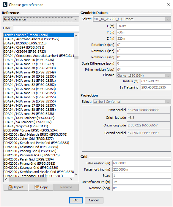
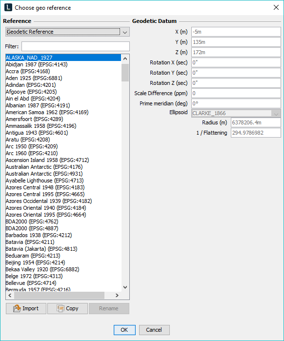
When you are selecting a reference system, you can select a predefined reference system from the list, or you can import a reference system from a file. To import a reference system from a file, click the Import button under the list.
The parameters of the predefined reference system are shown in the section(s) next to the reference list. Note that you cannot edit the parameters of a predefined reference system. To customize a predefined reference system, select or import the reference system and click on the Copy button under the reference list. The parameters of the copied reference system are editable. To rename the customized reference system, use the Rename button. To create a custom reference system, copy any existing reference system from the list, enter the appropriate parameters as described in Specifying the geodetic datum and give the reference a name using the Rename button. When renaming a reference system you are asked to specify the name (Geodetic or Grid Reference), the Geodetic Datum and Ellipsoid.
- Map-centric Lucy
-
To specify a georeference system in map-centric Lucy, go to Projection → More….
Specifying the geodetic datum
When customizing or creating a geodetic reference you need to specify the parameters of the geodetic datum. The geodetic datum is an approximation of the shape of the earth based on an ellipsoid. A commonly used geodetic datum is World Geodetic System 1984 (WGS 1984). The following parameters apply to a geodetic datum:
-
X, Y, Z: the distances in meters that indicate the position shift relative to WGS_1984.
-
Rotation X, Y, Z: the angular rotations in arc seconds relative to WGS_1984.
-
Scale difference: the scale difference in parts per million. The scale of the geodetic datum equals (1 + scale difference/1000000).
-
Prime meridian: the prime meridian in degrees relative to the Greenwich meridian (typically 0°).
-
Ellipsoid: by default the ellipsoid WGS_1984 is selected. It is possible to select another predefined ellipsoid from the Ellipsoid drop-down list or to define an ellipsoid by entering the values for the semi major radius (radius) and the inverse flattening (1/Flattening). Sometimes an ellipsoid is defined by the semi major radius (a) and the semi minor radius (b). The inverse flattening (1/f) is then defined as:
\[1/f = \frac{a}{a - b}\]When customizing or creating a grid reference you can select a predefined geodetic datum from the Select drop-down list or define a custom geodetic datum by selecting Custom from the list. For a customized geodetic datum you need to specify the same parameters as for a geodetic reference as described above. Additionally you need to define settings for the:
-
Projection: the projection that is used to project the data from the selected ellipsoid on a flat surface. You can specify one of the following parameters (depending on the chosen projection): the azimuth, the original latitude and longitude, the central meridian, the standard parallel, the first and second parallel, the pole, the perspective distance, and whether or not to consider the height. Changing the map projection provides more information about setting the map projection.
-
Grid: the false easting and false northing in the specified unit of measure, the scale, the unit of measure (a factor to convert the values to meters, for example 0.001 for millimeters) and rotation (in radians).
Saving a georeference system
To save a georeference system to file and use it for one or all data files located in the same directory, use the Tools→ Create geo reference file menu item. A dialog box allows you to select the georeference system and define the related settings as described above.
Click on the OK button at the bottom of the dialog box to save the defined georeference system in a file with the extension .epsg, .prj, or .ref. To use a .ref file for all data files in the same directory, enter the file name directory.ref. To use the .ref file for one data file (for example world.shp), give the .ref file the same name as the data file (world.ref).
Changing colors
Lucy provides the color selector as described in The color selector when you want to change the colors of:
-
The map background as described in Changing the map background color (Lucy GXY)
-
The map overview as described in Getting a map overview (Lucy GXY)
-
Layer data and labels as described in The layer properties panel
-
Shapes as described in Changing the shape style
When you are changing the colors of data such as pressure, temperature or elevation, you can use the color bar as described in The color bar.
The color selector
When you are changing the colors of the map or of map objects, you can select the colors from a color selector dialog box. Figure 44, “The color selector on a Windows client” shows the color selector on a Windows client.
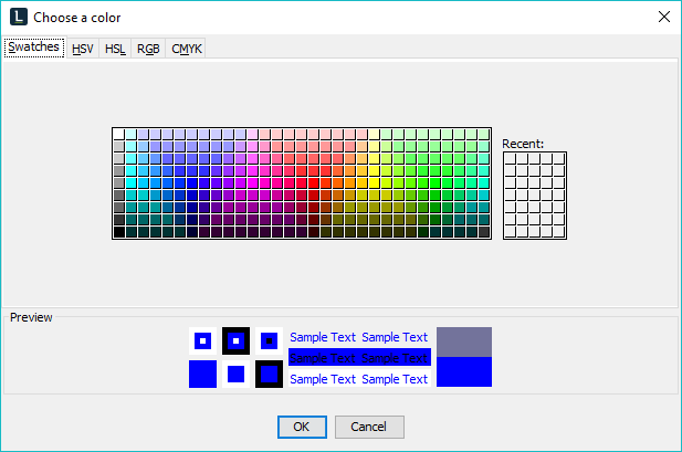
|
Note that the color selector looks different on Linux platforms. |
-
Swatches: allows you to select a color from the color swatch and preview it in the Preview pane before selecting it.
-
HSV: allows you to set the hue, saturation, and value of the selected color and the RGB values (see also the RGB tab).
-
HSL: allows you to set the hue, saturation, and lightness of the selected color and the RGB values (see also the RGB tab).
-
RGB: allows you to set the relative values of red, green, and blue of the selected color.
-
CMYK: allows you to set the values of the cyan, magenta, yellow and key (black) color components of the selected color.
With the Transparency slider you can specify the transparency of objects or make objects opaque. The Transparency preview section shows the selected setting.
To accept the selected settings, click on OK. To close the window without making changes, click on Cancel.
The color bar
To change the display colors of data such as pressure or temperature, an additional color bar is available on the Paint style tab in the layer properties panel. It displays a color bar as shown in Figure 45, “The color bar for pressure in a layer properties panel on a Windows client”. On 2D maps in Lucy GXY, you can also modify the display colors of elevation data layers with this color bar. To modify elevation colors in Lucy, see Setting elevation colors (Lucy).
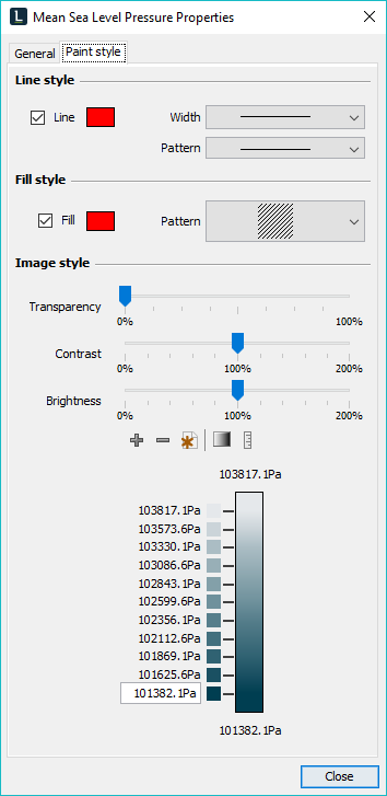
To change all settings, click on the ![]() icon above the color bar. A dialog pops up that allows you to set the minimum and maximum value and the delta of the intervals.
To change the settings of individual values, select the value in the color bar by clicking on the arrow next to it. The defined
value appears in a text box in which you can enter a new value or you can drag the arrow with the mouse to the new value.
The color icons allow you to change the display color of the individual value. Click on the color icon left of the arrow to
open the color selector and change the color as described in The color selector. To use gradient colors instead of distinct colors to represent the defined values, click on the gradient icon
icon above the color bar. A dialog pops up that allows you to set the minimum and maximum value and the delta of the intervals.
To change the settings of individual values, select the value in the color bar by clicking on the arrow next to it. The defined
value appears in a text box in which you can enter a new value or you can drag the arrow with the mouse to the new value.
The color icons allow you to change the display color of the individual value. Click on the color icon left of the arrow to
open the color selector and change the color as described in The color selector. To use gradient colors instead of distinct colors to represent the defined values, click on the gradient icon![]() above the color bar. To remove a value level, select the level and click on the icon with the minus sign above the color
bar. To add a level, select the level above which the new level should be added and then click on the icon with the plus sign.
above the color bar. To remove a value level, select the level and click on the icon with the minus sign above the color
bar. To add a level, select the level above which the new level should be added and then click on the icon with the plus sign.
Undoing and redoing actions
It is possible to undo and redo actions such as moving or editing an object or layer. It is not possible to undo or redo changes such as defining a georeference system or changing the map background color.
To undo the last action either:
-
Click on the Undo
icon in the map toolbar.
-
Select the Edit→ Undo menu item.
-
Press Ctrl+Z.
To redo the last undone action either:
-
Click on the Redo
icon in the map toolbar.
-
Select the Edit→ Redo menu item.
-
Press Ctrl+Y.
The last action performed is shown next to the Undo and Redo items in the Edit menu.
Working with maps
This article describes how you you can change the map projection, the coordinate system, the map background color, the map scale, add and remove grids to the map, define an area of interest, enable label decluttering, visualize magnetic north declination lines, measure distances, and use the raster scale.
Changing the map projection
To change the current projection of the map, select the Map→ Projection menu item or open the drop-down box next to the projection box in the map toolbar. You can choose one of the following commonly used projections:
-
Equidistant Cylindrical
-
Lambert Conformal
-
Lambert Azimuthal Equal Area
-
Mercator
-
Pseudo Mercator
-
Orthographic
-
Polar Stereographic (North)
-
Polar Stereographic (South)
-
Stereographic
-
Transverse Mercator
Additional projections are available through the Map→ Projection→ Edit Current menu item. The dialog box that appears is the same as the dialog to specify a georeference, as explained in Specifying the georeference system.
|
Note that when you have selected one of the additional projections, the chosen projection will not be added to the projection box in the map toolbar and the Map→ Projection menu. |
- Map-centric Lucy
-
To change the current projection in map-centric Lucy, select a projection from the Projection menu.
Specifying the georeference system provides more information on the Geodetic Datum, Projection, and Grid sections.
Adding and removing grids
The menu Map→ Grid allows you to add one of the following grids to the map view:
-
Lon Lat grid: the most commonly used grid. A longitude-latitude grid is formed by evenly spaced meridians and parallels.
-
MGRS Grid (Military Grid Reference System): divides the earth into grid zones that are refined depending on the view scale. This functionality requires the Defense Symbology component.
-
Georef Grid (World Geographic Reference System): is essentially based on the geographic system of latitude and longitude, but uses a simpler and more flexible notation.
-
XY Grid: a Cartesian (XY) grid is formed by evenly spaced meridians and parallels.
On 2D maps in Lucy GXY, you can add one of the following grids:
-
Georef Grid (World Geographic Reference System)
-
MGRS Grid (Military Grid Reference System) : divides the earth into grid zones that are refined depending on the view scale. This functionality requires the Defense Symbology component.
-
Border Grid: longitude and latitude displayed on the four borders of the view
-
XY Grid: a Cartesian (XY) grid is formed by evenly spaced meridians and parallels.
The selected grid is added to the layer tree and displayed in the map view. To remove the grid, select it in the layer tree and click on the Delete icon in the layer toolbar or right-click in the layer tree and select Delete layer from the pop-up menu.
Changing the coordinate system
By default the coordinates of the current mouse position are shown at the bottom of the map in the coordinate system of the selected layer. To change the coordinate system of the mouse coordinates, select Edit→ Point Format.
To view additional coordinate settings, select the Tools→ Grid Coordinate menu item. The Grid Coordinate panel appears top left of the map view with the following sections:
-
Map Control: The Map box shows for which map the coordinate information is displayed and allows you to select another map if more than one map is open. The Mode box shows for which map action the coordinate information is updated: a mouse click, a mouse move, or a selection of an object.
-
Location: The longitude and latitude coordinates of the current mouse position.
-
Coordinate: The coordinates in different formats (DMS(1), DMS(2), UTM, GeoRef, UPS) and the UTM zone. DMS stands for Degrees, Minutes and Seconds. DMS(1) uses the + and - sign to indicate the North, South, West, or East whereas DMS (2) uses N, S, W or E.
-
Datum: The Name box shows the geodetic datum. The Ellipsoid box shows the ellipsoid that is used for the selected geodetic datum.
|
Note that the Grid Coordinate panel allows you to view the current coordinate settings, not to change any of the settings. |
Figure 46, “The Grid Coordinate panel” shows the Grid Coordinate panel. Specifying the georeference system provides more details on the coordinate systems and the related settings.
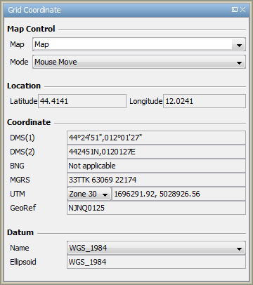
Visualizing the magnetic north declination
The magnetic north declination is the angle between the magnetic north of a point on the earth and the true north. The magnetic north is the bearing as indicated on a compass and changes depending on the location and date. The true north is the bearing to the geographical north pole (Latitude = 90°). The declination is positive if the magnetic north is east of the true north and negative if the magnetic north is west of the true north.
Lucy offers two possibilities to visualize the magnetic north declination on the map:
-
The magnetic north declination tool shows the magnetic north declination in a small box on the map next to the mouse pointer. To activate the tool, select the Map→ Controls→ Magnetic North Declination menu item. If no layer with magnetic lines is available, the tool uses the default settings to calculate the magnetic lines (WMM as geomagnetic model and today as date). If layers with magnetic lines are available, the tool uses the upper layer with magnetic lines. When moving the mouse over the map, the magnetic north declination value in the text box automatically adapts to the mouse position. Click on the map to rotate the map in the direction of the magnetic north. Right-click on the map to undo the rotation.
-
The magnetic north declination panel allows you to calculate and define the lines of the constant magnetic north declination for a specific date, add the lines to a new layer, and display them on the map. To open the magnetic north declination panel, select the Tools→ Magnetic North Declination menu item. A panel appears as shown in Figure 47, “The Magnetic North Declination panel”. The magnetic north declination panel provides detailed information on the fields in this panel. Figure 48, “A map with magnetic north declination lines” shows a map with magnetic north declination lines.
The magnetic north declination panel
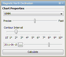
The magnetic north declination panel contains the following properties:
-
The (geo)magnetic model used to calculate the magnetic north declination lines. Options are the World Magnetic Model (WMM) and the International Geomagnetic Reference Field (IGRF) model.
-
The precision of the lines against the speed of the calculation. The more precise the lines are, the slower the calculation will be, and the faster the calculation is, the less precise the lines will be.
-
The number of degrees between the lines.
-
The date. To change the date, either enter a date in the box or drag the slider. The date range depends on the chosen (geo)magnetic model.
Click on the Calculate button to calculate the magnetic north declination lines as defined in the panel. A layer for the lines is added to the layer tree and the lines are displayed on the map. Figure 48, “A map with magnetic north declination lines” shows a map with magnetic north declination lines. On the black line the magnetic north declination is 0, the brown lines have a negative magnetic north declination, and the blue lines have a positive magnetic north declination.
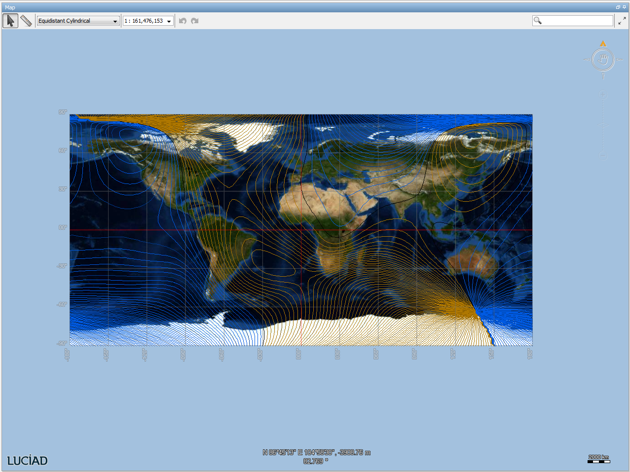
Measuring distances on the map
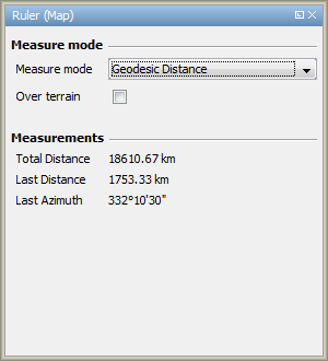
The Ruler tool as described in The map tools allows you to measure distances on the map. When the Ruler tool is active, you can draw shapes on the map as described in Drawing shapes on the map. Usually the Ruler tool is used for measuring the path between objects on the map. In that case it may be useful to make the layer with the objects Snappable so that the path will automatically snap to objects on the map. The layer tree popup menu describes how to make a layer snappable.
When the Ruler tool is active, the Ruler panel is displayed top left of the map view. The panel shows the measurement mode settings and the actual measurements of the last created path. Select one of the following measurement modes from the drop-down list:
-
Geodesic Distance, measures distances ``as the crow flies''. The geodesic distance mode measures the shortest distance between two points, taken the curvature of the Earth into account. It is also known as the distance of a great circle or orthodrome, measured on the ellipsoid.
-
Rhumbline Distance, typically used to measure the shortest distance between two points for objects traveling over long distances with the aid of a compass. A rhumbline distance measurement maintains a constant compass bearing, and is used to plan airplane flights or boat voyages, for instance. It is also known as the distance of a loxodrome, measured on the ellipsoid
-
Cartesian Distance, measures the distance between two points, disregarding the curvature of the Earth, in the projected coordinate system of the map. It is similar to using an actual ruler, and appropriate for measuring smaller-scale objects like trees and buildings. You would get the same result if you pointed a laser device to make measurements. In Lucy GXY, this measurement mode is called Projection plane distance.
|
If you map displays terrain elevation, your Cartesian distance measurement lines may be partially obscured by the terrain. This does not affect the accuracy of the measurement in any way. |
The measurements section shows:
-
Total Distance: the total distance of the path
-
Last Distance: the distance between the last two points of the path
-
Last Azimuth: the azimuth from the second last point to the last point of the path, only available on 2D maps in Lucy GXY.
- Map-centric Lucy
-
To measure distances in map-centric Lucy, click the Ruler icon in the side tool bar.
Changing the scale of the map
If you cannot see the scale box, choose a projection different from 3D in the projection selection drop-down menu.
The scale box in the map toolbar displays the scale in which the current map is displayed in the map view. The scale is calculated based on the center of the view. So if the view changes, the center and thus the scale changes as well. This is contrary to paper maps where the scale is based on the center of the projection and does not change. To change the map scale, select one of the options from the drop-down list or enter a value in the scale box. When you enter a value in the box you can use both a colon or a slash as separator.
The scale icon in the bottom right corner of the map view is related to the scale box. The length value refers to the actual length of the scale icon expressed in the current distance unit. Setting units, formats, and the coordinate system provides more information on the settings of measurement units. To hide the scale icon in the map view, deselect the Map→ Show Scale menu item.
|
The map scale will automatically be adjusted when zooming in or out on the map, panning the map, and changing the projection of the map. |
Figure 50, “The map scale drop-down list” shows the drop-down list of the scale box and the scale icon in the bottom right corner of the map view.
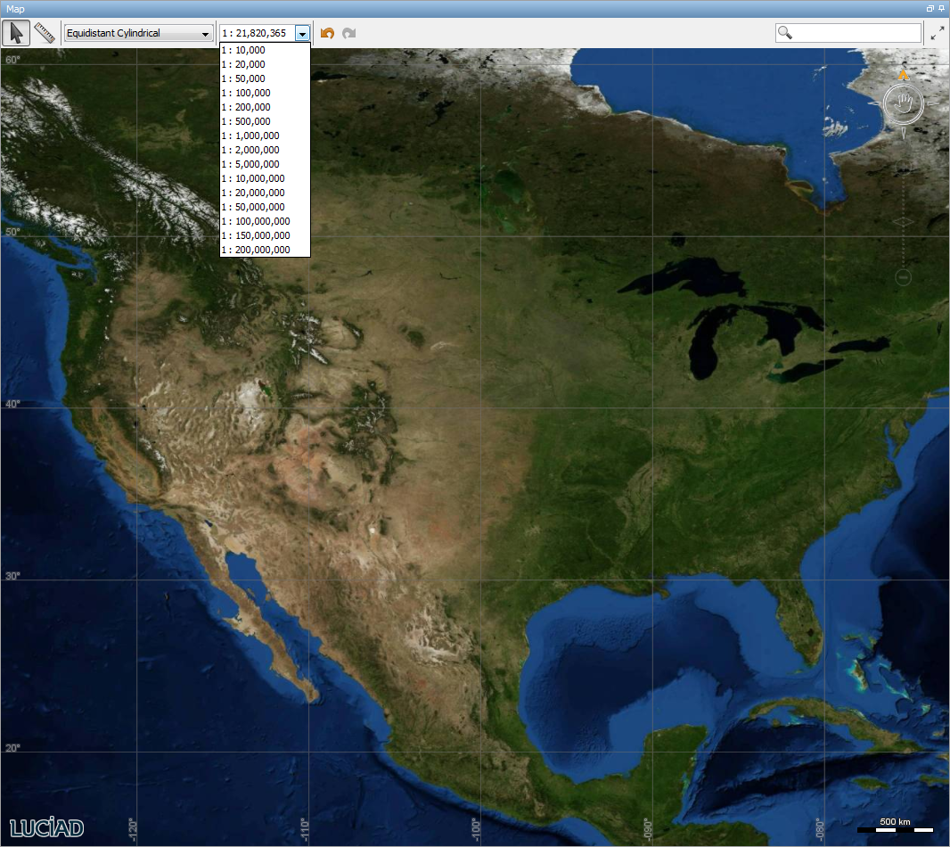
- Map-centric Lucy
-
To hide the scale bar in map-centric Lucy, go to View → Show Scale, and deselect the option.
Finding places and data on the map
The search box in the tool bar allows you to find places and particular layer data on the map. You can enter:
-
Coordinates: decimal coordinates or latitude/longitude coordinates.
-
Place names: country, city and landmark names.
-
Data properties: terms that possibly match the properties of the data in one of the layer data sources.
|
Lucy searches all the data in the layer data source, even the data that is currently not loaded on the map. |
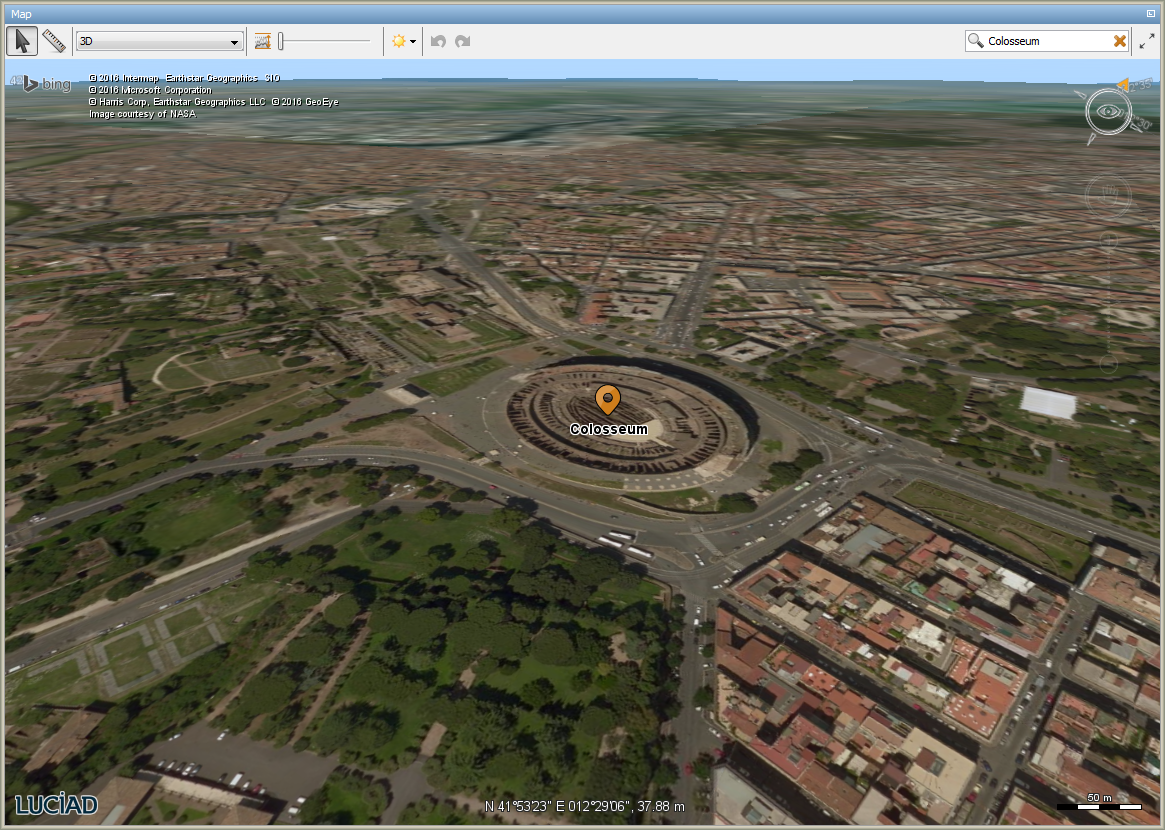
Lucy uses search services to retrieve matches for the search terms you enter. If multiple matches are found, you can select the right match from a drop-down menu.
Press Enter, and the map will automatically fit to the area with the selected search result. The exact location is indicated with a placemarker. If the search result belongs to the data loaded on the map, the appropriate data object is selected on the map.
Comparing data visually (Lucy)
It can be difficult to spot minute visual differences or similarities between data sets, for instance between two images captured at the same location but at different times. To make visual data comparison easier, Lucy allows you to compare map layers by visualizing them side-by-side or in quick succession.
Swiping to compare layers side-by-side
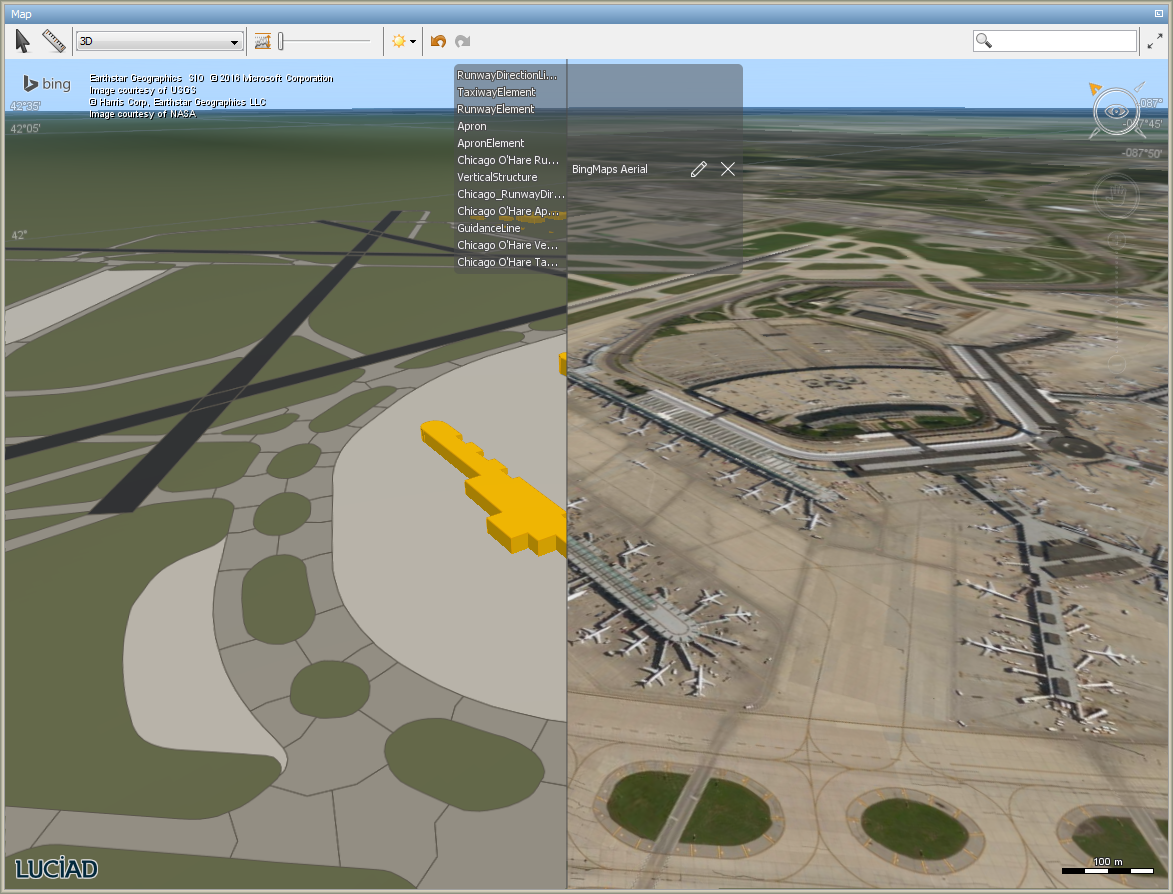
To compare data by swiping between two side-by-side layers:
-
Select Map → Controls → Swipe.
-
In the Choose layers to compare dialog, select the layers that you want to compare. You can select multiple layers in each column of the dialog.
-
Click OK. Lucy displays a swipe line across the map view. The label at the top of the swipe line indicates the layers that are visible on each side. The layers you selected in the left column of the dialog are visible on the left of the swipe line, while the layers selected on the right appear on the right of the swipe line.
To change the orientation of the swipe line from vertical to horizontal, drag the swipe line up or down. Drag it to the left or right to change the orientation to vertical again.
- Map-centric Lucy
-
To swipe between layers in map-centric Lucy, click the Eye icon in the side tool bar, and select the Swipe option.
Toggling layers to compare data
To compare data by quickly swapping map layers in the map view:
-
Select Map → Controls → Toggle.
-
In the Choose layers to compare dialog, select the layers that you want to toggle. You can select multiple layers in each column of the dialog.
-
Click OK. Lucy displays only the layers you selected in the left dialog column.
-
Click the map view to swap those layers for the layers selected in the right column of the dialog.
-
Keep clicking to rapidly toggle the selected layers. The label at the top of the map view displays which layers are currently visible.
- Map-centric Lucy
-
To toggle layers in map-centric Lucy, click the Eye icon in the side tool bar, and select the Toggle option.
Inspecting data through a layer porthole
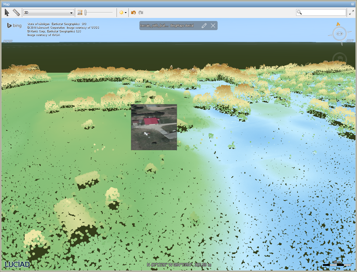
To compare data by overlaying layers, and inspecting a data layer set through a porthole cut in the data layers on top:
-
Select Map → Controls → Porthole.
-
In the Choose layers to compare dialog, select the layers that you want to cut through in the left dialog column. In the right dialog column, select the layers that you want the porthole to expose.
-
Click OK. Lucy displays a porthole around the mouse position. The porthole area displays your layer selection from the right dialog column. On the rest of the map, Lucy displays the layers selected in the left dialog column. The label at the top of the map view displays the layer selection you made.
To move the porthole, move the mouse around the map.
To change the size of the porthole, press and hold the Shift key while scrolling the mouse wheel up or down.
You can peel off layers in the porthole only, and still display all layers in the rest of the view. To do so, select just the layer that you want to peel off in the left column of the Choose layers to compare dialog. Do not select any layers in the right dialog column. As a result, the porthole peels off the selected layers, but still displays the other layers. The rest of the view displays all layers.
- Map-centric Lucy
-
To inspect layers through a porthole in map-centric Lucy, click the Eye icon in the side tool bar, and select the Porthole option.
Changing or stopping data comparison
To change the layer selection, click the Pencil icon on the swipe line/toggle/porthole label. You can re-define your layer selection in the Choose layers to compare dialog.
To stop comparing layers and return to the regular map view, select the X icon on the swipe line/toggle label.
Magnifying part of the map
To magnify a part of the map, go to Map→ Controls, and select the Magnifier tool. Click on the map to see the Magnifier window as shown in Figure 54, “The magnifier window”. You can move the magnifier window over the map by dragging the mouse.
To zoom in and out within the magnifier window, press and hold the Shift key while scrolling the mouse wheel up and down.
To change the size of the magnifier window, press and hold the Ctrl key while scrolling the mouse wheel up and down.
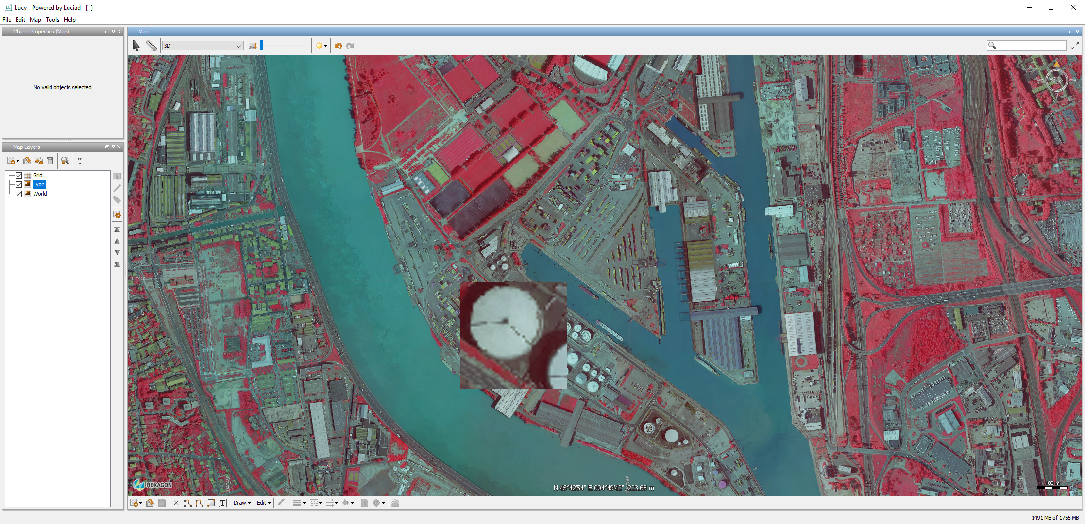
To close the magnifier, select the Navigate and select controller from the map tool bar or the Controls sub-menu.
Controlling the light on your map (Lucy)
Lucy allows you to mimic the presence and absence of sunlight on your map. In addition, you can control the position of the sun, and position it to light up the map from your viewing perspective, or simulate a certain time of day.
By default, the entire map is lit. To change the lighting, click the sun icon on the map toolbar, and select the appropriate option from the drop-down menu:
-
To keep the entire map lit, select the No Lighting option. No lighting scheme is set. The entire globe surface is equally bright, regardless of your perspective on the map, or the time of day.
-
To let sunlight illuminate the map from your perspective of the map, select the Automatic option. The part of the map you are viewing is lit, as if you were looking from the sun, while the outer edges of the focus area gradually darken.
-
To mimic the sunlight at a particular time of day, select the Time of Day option. Use the slider to select a time of day, and select the time zone in which the selected time is valid from the menu. If you set the time to 23:59 in a GMT+1 time zone, for example, and look at Europe, the map will be dark.
- Map-centric Lucy
-
To control the map lighting map-centric Lucy, click the Sun icon in the top tool bar.
Setting elevation colors (Lucy)
To represent elevation data, Lucy maps levels of elevation to a range of colors in a color gradient. The elevation color range set by Lucy is a global one: each set of elevation data in the application is mapped to the same color range. A specific elevation level is displayed in identical coloring in each layer.
Lucy comes with a suggested elevation-to-color mapping, which you can easily customize to your needs.
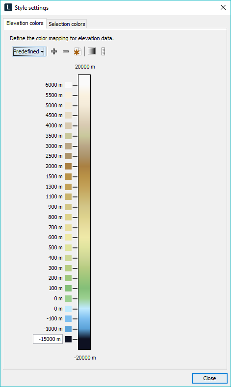
The elevation color mapping consists of a set of elevation levels tied to a specific color. As the mapping moves from one elevation level to another, the colors gradually change along the gradient.
To customize the elevation color mapping, go to Map→ Style settings…. The Elevation colors tab displays a gradient editor for the default elevation color model.
If you want to change elevation colors on 2D maps in Lucy GXY, you must do so at the layer level. A color bar for changing elevation colors is available on the Colors tab of the layer properties panel for elevation data layers.
- Map-centric Lucy
-
To set elevation colors in map-centric Lucy, go to View → Style settings….
Changing elevation colors
To make a particular elevation level stand out from the others, you can assign a different color to it. This can even be a color that falls completely outside the color gradient. To change the color of an elevation level, click the colored squares next to the elevation levels, and select a color from the Choose Color dialog.
You can also re-assign a color to a different elevation. To do so, select the elevation specified next to the color, and type in the required elevation. When you press ENTER, the color and the elevation specification move to the requested position on the gradient.
Increasing or decreasing the elevation range
You can re-define the extent of your elevation color model. You can stretch it to include higher and lower elevations, or you can shrink the extent and introduce more color variation within a smaller elevation range.
To re-define the extent of the color model, select the ![]() icon, and enter new minimum and maximum levels. The Delta field allows you to specify the elevation intervals between color transition points. If you set a delta of 50 m, for example,
the elevation color will change every 50 meters.
icon, and enter new minimum and maximum levels. The Delta field allows you to specify the elevation intervals between color transition points. If you set a delta of 50 m, for example,
the elevation color will change every 50 meters.
Inserting and removing elevation levels
To add an elevation level within the color gradient and assign a color to it, select the elevation level right above the level
you want to give a color, and click the  icon. A new elevation level is added and assigned a color along the gradient.
To remove an elevation level, select it and click the  icon.
icon.
Tweaking color transitions
To distinguish more clearly between elevation levels, you can switch off the smooth color progression in the color model,
and display sharp color transitions where elevation levels change on the map. To switch smooth color progression on or off,
click the ![]() icon.
icon.
To display the elevation color map on a linear scale, click the  icon. In the linear scale view, you can increase or decrease the elevation range covered by a specific color. Drag the sliders
next to the elevations up or down to the required color transition points.
icon. In the linear scale view, you can increase or decrease the elevation range covered by a specific color. Drag the sliders
next to the elevations up or down to the required color transition points.
Changing the map background color (Lucy GXY)
To change the background color of a 2D map, select Map→ Colors→ Background menu item and select a color from the color selector as described in The color selector.
Defining an Area of Interest (Lucy GXY)
The default Lucy interface contains an Area of Interest (AOI) layer. This layer has some predefined areas of interest that allow you to display a specific area on the map and to limit map operations to that area. Figure 56, “The default Area of Interest in the map view and the Map Overview panel” displays the AOI with a yellow rectangle in the map view.
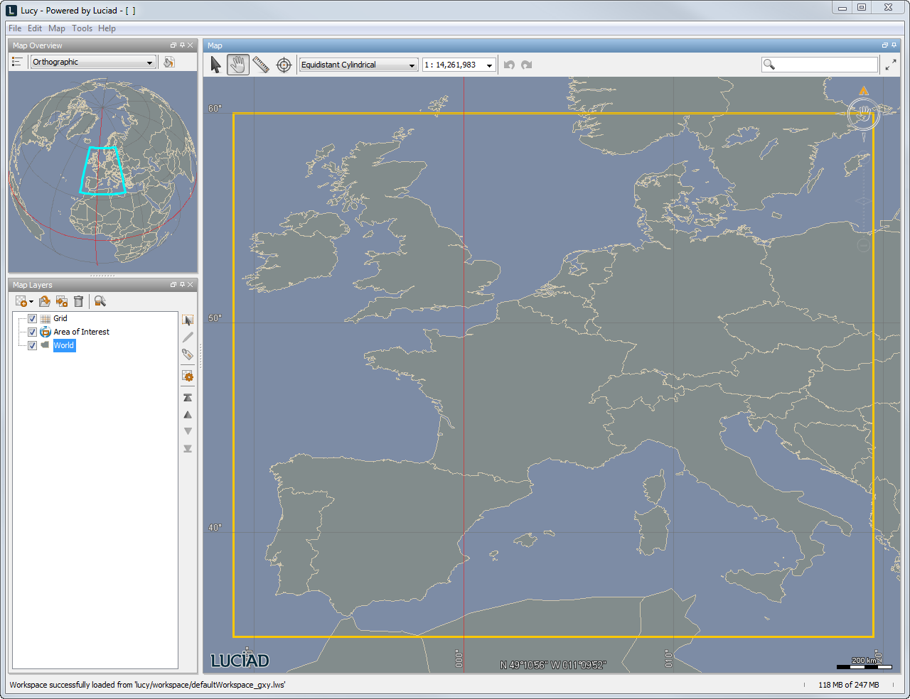
To change the default AOI to one of the other predefined areas, select an AOI from the Map→ Area of Interest menu, for example United States. The selected AOI becomes active and both the map view and Map Overview are scaled to the selected AOI as shown in Figure 57, “The United States as Area of Interest”. The blue rectangle represents the AOI and indicates that the AOI is selected.
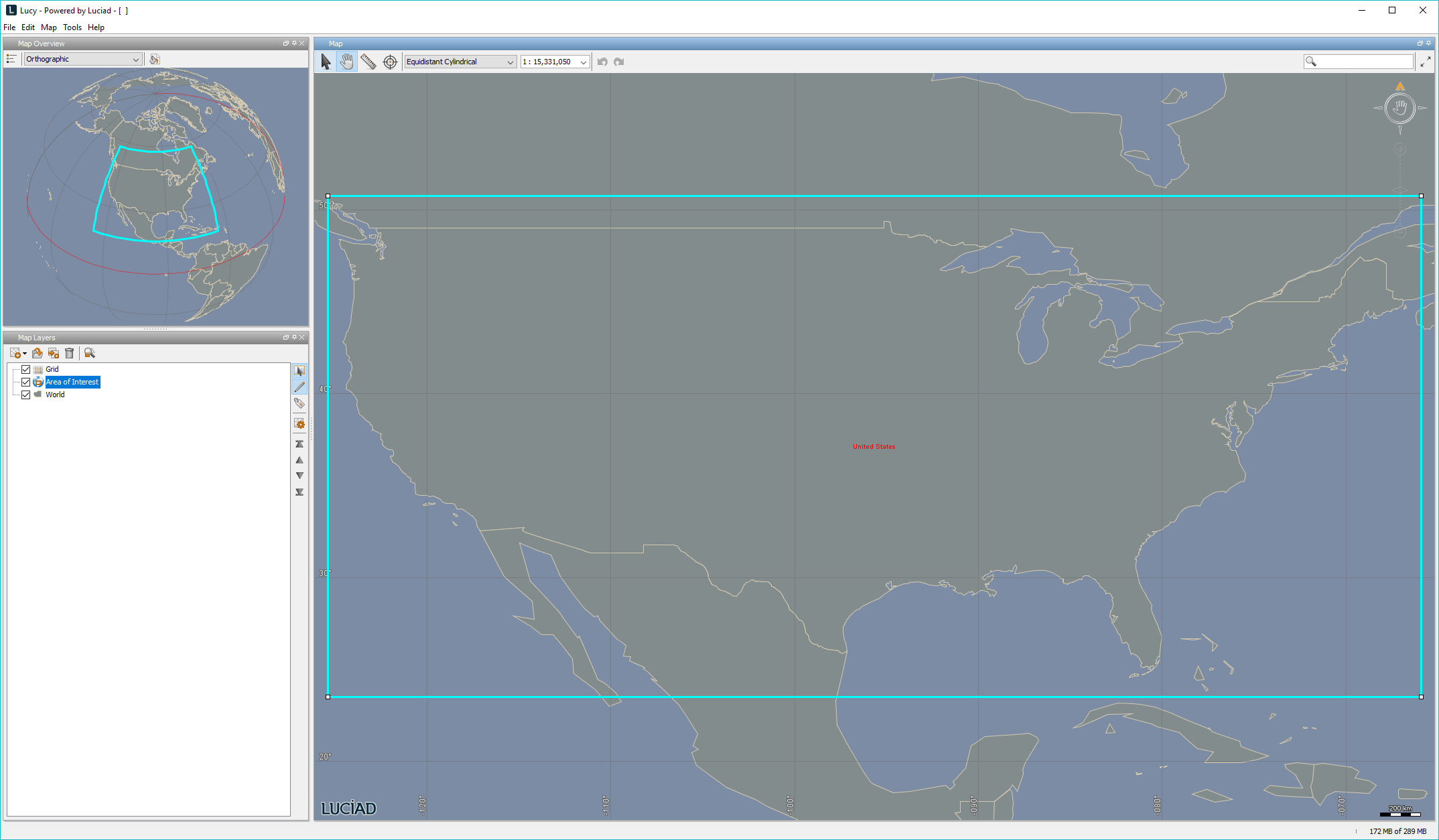
The other options of the Map→ Area of Interest menu allow you to:
-
Show all predefined areas of interest.
-
Fit the active AOI to the map view.
-
Fit the active AOI to the selected layer that is displayed on the map.
To create a new AOI, select the Map→ Area of Interest→ New Area of Interest menu item. The new AOI is selected in the map view. Use the left mouse button to drag the AOI to a new location and to resize it if needed.
To change the properties of the active AOI, select the AOI in the map view, right-click, and select the Properties option. The Object properties panel appears in the top left corner of the application window. This panel allows you to define the following values for the selected AOI:
-
Name: The name of the AOI as shown in the map view and in the Map→ Area of Interest menu.
-
Description: A short description of the AOI.
-
Scale: If a scale is specified, the map shows the AOI in the specified scale. When navigating to an AOI on the map, the map scales to fit to the specified scale of the AOI.
-
Center, Width, Height: The coordinates for the center of the AOI and the coordinates from the center that define the width and the height of the AOI. Use this option to define the size of the AOI relative to the center.
-
North West Location, South East Location: The coordinates of the top left corner and the bottom right corner of the area. Use this option to define the size of the AOI by its corner points.
Figure 58, “The Object properties panel of the United States as Area of Interest” shows the Object properties panel of the United States as AOI.
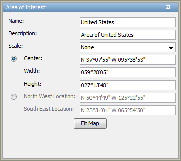
To delete an AOI, select the AOI in the map view, right-click, and select the Delete option. Note that the AOI is not only deleted from the map view but also from the Map→ Area of Interest menu.
Enabling global label decluttering (Lucy GXY)
|
In general, Lucy declutters labels automatically. On 2D maps in Lucy GXY, however, you must activate global label decluttering manually. |
When there are many labels on the map, when labels are large, or when labeled objects are close to each other, the labels might overlap each other. To prevent label overlap for all labels on the map, select Map→ Global label decluttering. All map labels will then automatically rearrange on the map to avoid overlap with other labels. If necessary, some labels might disappear. Figure 59, “A map with cluttered labels” shows a map with cluttered labels and Figure 60, “A map with decluttered labels” shows the same map with decluttered labels.
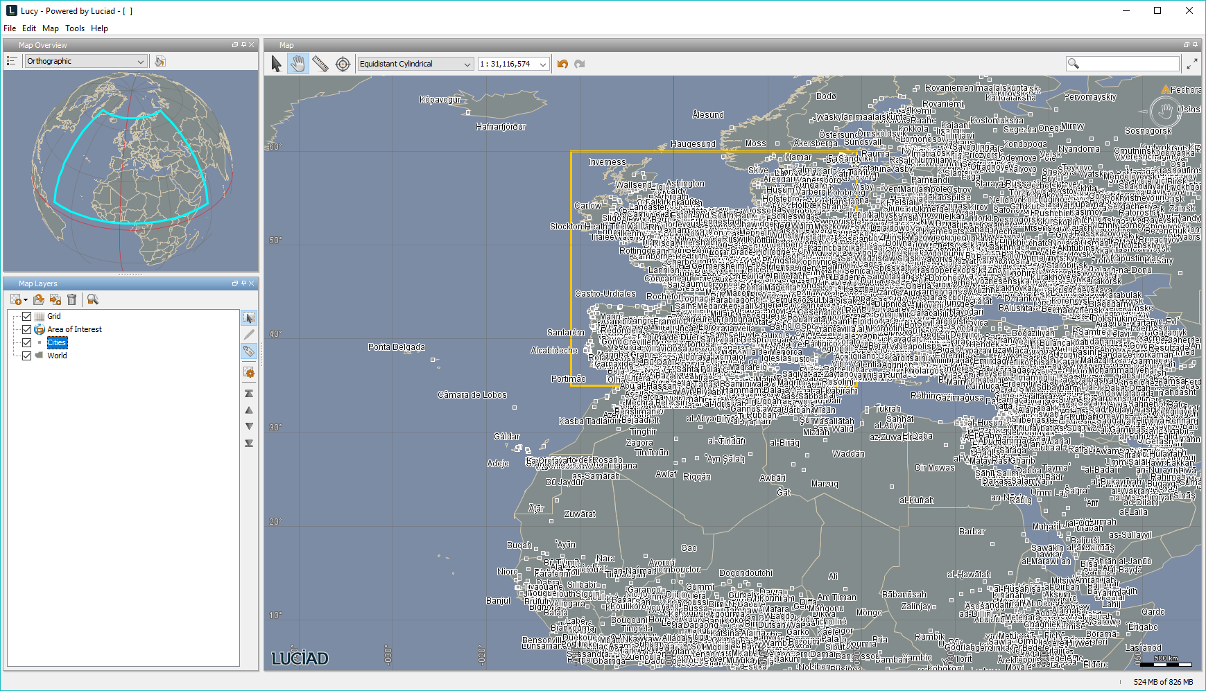
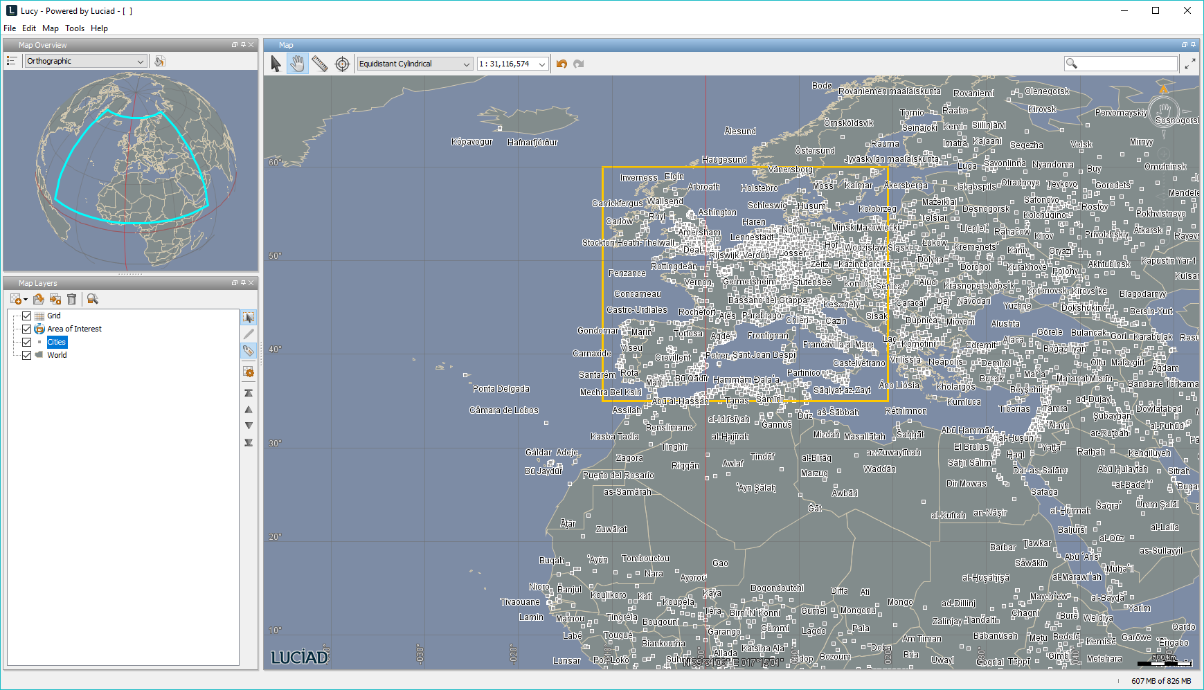
Using the raster scale (Lucy GXY)
When zooming in on raster data on a 2D map, you can display a scale on the map showing the available raster levels and the zoom level by pressing the Ctrl-key. The raster scale allows you to zoom in or out to a specific raster level as shown in Figure 61, “The raster scale indicating the raster levels and the zoom level”. The black lines represent the available raster levels and the orange line represents the zoom level. By zooming in or out the zoom level snaps to the nearest raster level.
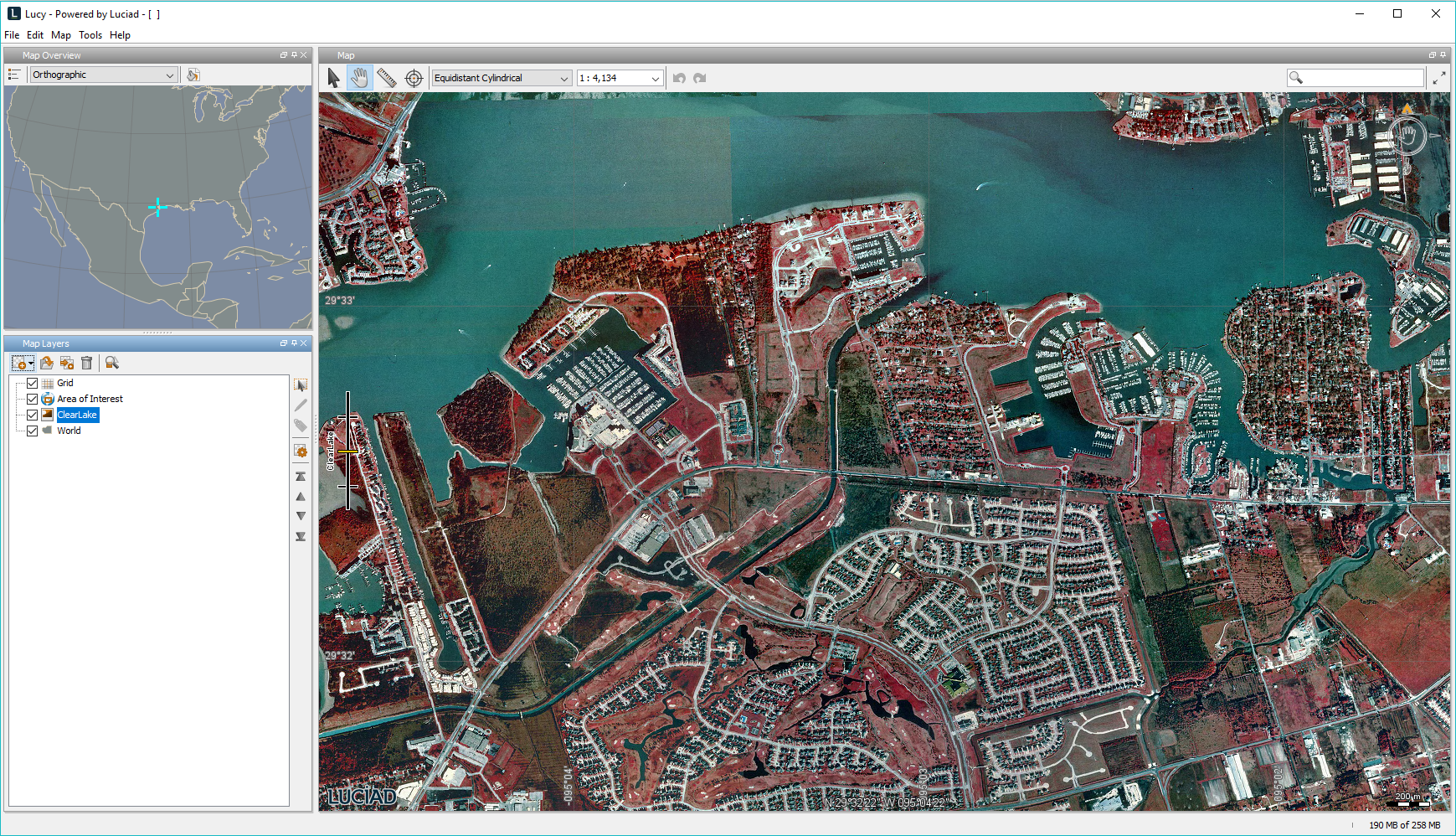
The scale will only show available levels of raster data. When no raster data is loaded, a message indicates that no raster is found.
Drawing shapes on the map
Lucy facilitates the drawing of shapes on the map such as points, rectangles, (poly)lines, buffers and many other shapes. Shapes allow you to connect objects in the map view with each other, for example, or create areas with specific properties. Shapes are added to a separate drawing layer which you can manipulate the same as any other map layer as described in Working with layers. This article describes which shapes you can create with Lucy and the actions you can perform with shapes.
Adding a drawing layer
You can only draw shapes on the map if a drawing layer is present in the layer tree. If no drawing layer is present you can create and add one either by:
-
Clicking on the Add layer icon
in the layer control toolbar.
-
Selecting the File→ New→ Layer menu item.
-
Selecting the Map→ Drawing bar menu item.
- Map-centric Lucy
-
To start drawing in map-centric Lucy, select one of the drawing icons in the side tool bar. A message box will ask you to confirm that you want to create a drawing layer.
If a dialog box for layer type selection appears, select the layer type Drawing, and click OK. The Create a new Drawing layer dialog box opens, as shown in Figure 62, “The dialog box for creating a new drawing layer”.
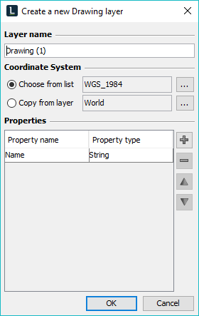
This dialog box for creating a new drawing layer allows you to define:
-
Layer name: the name of the layer. After creating the layer, you can change the layer name in the layer properties panel, as described in The layer properties panel.
-
Coordinate system: the coordinate system to use for the shapes of the drawing layer. You can accept the default coordinate system (WGS_1984), select a coordinate system of your choice or copy the coordinate system of an existing layer. To choose a coordinate system, click the dotted icon next to the text box of the Choose from list option. The dialog box described in Specifying the georeference system appears. It allows you to choose a coordinate system. To copy the coordinate system of an existing layer, click the dotted icon next to the text box of the Copy from layer option. A dialog box will let you choose the layer. The coordinate system of the selected layer will be reused for the drawing layer. After creating a layer, you can no longer change the coordinate system of the new layer.
-
Properties: Generic shape attributes assigned to the shapes in the drawing layer. You can define properties that apply to all types of shapes in the drawing layer. Each shape created in the drawing layer will let you set a value for the properties you create here. You can give each shape you draw a name, for instance, by filling in a string value for the name property. These generic properties differ from the individual shape properties, such as location, distance, and altitude, which are specific to a type of shape. To add a new generic property, click on the plus icon next to the property list. Give the new property a name and select its type: String, Integer, Double, Boolean or Date. To delete a property from the list, click on the minus icon. Use the arrow keys to rearrange the properties in the list. Once you close this dialog box, the layer is created, and you can no longer change the properties of the layer.
Click OK to finish layer creation. The layer tree contains the new drawing layer, and a drawing toolbar is added under the map as shown in Figure 63, “The drawing toolbar”. To hide the drawing toolbar, deselect the Map→ Drawing bar menu item.

- Map-centric Lucy
-
To access the drawing options in map-centric Lucy, see the side tool bar. It stacks roughly the same options as the Lucy drawing bar.
Drawing shapes on the map
You can only draw shapes on the map if a drawing layer is present in the layer tree. If the layer tree does not contain any drawing layers, add a drawing layer as described in Adding a drawing layer. If multiple drawing layers are present, select one drawing layer. New shapes will be added to the selected drawing layer.
The drawing toolbar contains shape icons and a shape list that allow you to draw all kinds of shapes on the map. This section describes the different shapes, the shape properties, and the actions that you can perform with the created shapes. The description applies to shapes drawn on 2D as well as on 3D maps. Differences between drawing on 2D maps and drawing on 3D maps will be explained.
|
While drawing a shape on a 2D map, you can undo an insertion by pressing the Backspace key. To cancel the drawing, press the Esc key. |
On a 3D map, the drawing toolbar contains an icon to enable the Terrain Following Mode (TFM): ![]() . When an object is created and TFM is enabled,
. When an object is created and TFM is enabled, ![]() , the altitude of objects such as points or 3D polylines are automatically adjusted to the altitude of the underlying terrain.
When TFM is disabled, the altitude of the underlying terrain is ignored and the points have an altitude of 0 meters. When
TFM is enabled, the altitude of the object above the terrain is kept constant. If, for example, a point with an altitude of
5 meters moves to a mountain with a height of 3000 meters, the altitude of the point automatically adjusts to 3005 meters.
, the altitude of objects such as points or 3D polylines are automatically adjusted to the altitude of the underlying terrain.
When TFM is disabled, the altitude of the underlying terrain is ignored and the points have an altitude of 0 meters. When
TFM is enabled, the altitude of the object above the terrain is kept constant. If, for example, a point with an altitude of
5 meters moves to a mountain with a height of 3000 meters, the altitude of the point automatically adjusts to 3005 meters.
To use TFM on 2D maps, you need the Terrain Analysis Engine component.
Drawing shapes from the shape icons
This section describes which shapes you can create using the shape icons in the drawing toolbar and what the properties for each of these shapes are, as shown in the Object properties panel. Changing the shape properties describes how to change the properties of a created shape.
If the drawing toolbar is not visible, select the Map→ Drawing bar menu item. The drawing toolbar appears under the map.
|
Double-clicking a shape icon allows you to draw multiple shapes of the selected shape. A plus sign is added to the icon and after you have drawn one shape you can click on the map to draw another one. Click on the icon again to disable this option. |
Use the shape icons in the drawing toolbar to quickly draw one of the following shapes:
Drawing points
To create a point, click on the Create a point icon ![]() in the drawing toolbar. Click on the map to add the point to the map.
in the drawing toolbar. Click on the map to add the point to the map.
To create a point on a 3D map, click on the map to mark the point location, modify the point’s altitude by dragging the mouse up or down, and finish the point creation by clicking again.
To change the appearance of the point icon on the map, select the point and click on the Choose point icon ![]() on the drawing toolbar. Changing the shape style provides more information on changing the point shapes.
on the drawing toolbar. Changing the shape style provides more information on changing the point shapes.
The Object properties panel of a point shows the following properties: location and altitude.
Drawing polylines
To create a polyline, click on the Create a polyline icon ![]() in the drawing toolbar. Click on the map to indicate the start point of the polyline. Move the mouse and click on the map
to add extra points to the polyline. To add the end point to the polyline, double-click or right-click on the map. .
in the drawing toolbar. Click on the map to indicate the start point of the polyline. Move the mouse and click on the map
to add extra points to the polyline. To add the end point to the polyline, double-click or right-click on the map. .
|
For freehand drawing, click and hold down the left mouse button while moving the mouse. |
The Object properties panel of a polyline shows the following shape properties: a list with the individual points constituting the polyline, the location for each point, and the bearing and distance to the next point.
Drawing polygons
To create a polygon, click on the Create a polygon icon ![]() in the drawing toolbar. Click on the map to indicate the start point of the polygon. Move the mouse and click on the map
to add extra points to the polygon. To add the end point to the polygon, double-click or right-click on the map. The first
point will automatically be connected to the last point to close the polygon.
in the drawing toolbar. Click on the map to indicate the start point of the polygon. Move the mouse and click on the map
to add extra points to the polygon. To add the end point to the polygon, double-click or right-click on the map. The first
point will automatically be connected to the last point to close the polygon.
|
For freehand drawing, click and hold down the left mouse button while moving the mouse. |
The Object properties panel of a polygon shows the following shape properties: a list with the separate points of the polygon, the location, and the bearing and distance to the next point.
Drawing rectangles
To create a rectangle, click on the Create a rectangle icon ![]() in the drawing toolbar. Click on the map to indicate the start corner of the rectangle. Move the mouse and click on the map
to add the opposite corner to the rectangle.
in the drawing toolbar. Click on the map to indicate the start corner of the rectangle. Move the mouse and click on the map
to add the opposite corner to the rectangle.
The Object properties panel of a rectangle shows the following shape properties:
-
The coordinates of each corner point, identified as the North-West, North-East, South-West, and South-East corner points.
-
The width and height of the rectangle. The width indicates the length of the rectangle side going from one corner point Eastward or Westward to the other corner point. The height indicates the length of the rectangle side from one corner point going Northward or Southward to the other corner point. Figure 64, “The Object properties panel of a rectangle in a geodetic reference system” shows the width and height values of a rectangle created with a geodetic reference system. If a grid reference system is used, the values in degrees are not applicable. The width in Figure 64, “The Object properties panel of a rectangle in a geodetic reference system” shows the length in degrees and km of the side starting at the southwest corner and ending at the southeast corner. The height in Figure 64, “The Object properties panel of a rectangle in a geodetic reference system” shows the length in degrees and km of the rectangle side starting at the southwest corner and ending at the northwest corner. The values for the degrees and km depend on each other. If you change the value in km, for example, the value in degrees is automatically adjusted. If the rectangle is moved to another location, the degrees remain the same but the km values will be recalculated.
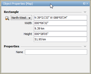
Drawing text
The Text icon ![]() allows you to add text to the map. Click on the map to indicate the location of the text, and type the text in the Object
properties panel, and press Ctrl+Enter. To change the font settings, click on the Font icon
allows you to add text to the map. Click on the map to indicate the location of the text, and type the text in the Object
properties panel, and press Ctrl+Enter. To change the font settings, click on the Font icon ![]() at the right side of the drawing bar. Changing the shape style provides more information on the different font options.
at the right side of the drawing bar. Changing the shape style provides more information on the different font options.
The Object properties panel of text shows the following shape properties: the location and the text. To change the current text, overwrite the current text with another text. Press Ctrl+Enter to apply the changes.
Drawing shapes from the Draw button list
This section describes which shapes you can create using the Draw button in the drawing toolbar and what the properties of each of these shapes are, as shown in the Object properties panel. Changing the shape properties describes how to change the properties of a created shape.
If the drawing toolbar is not visible, select the Map→ Drawing bar menu item. The drawing toolbar appears under the map. When you click on the Draw button in the drawing toolbar, a list with shapes pops up, as shown in Figure 65, “The list of shapes from the Draw button”.
|
All shapes on the shape list are available when a geodetic reference system is used. When a grid reference system is used, the following shapes are not enabled: parallel, meridian, rhumb polyline, rhumb polygon, dome, sphere, 3D buffer, and variable 3D buffer. |
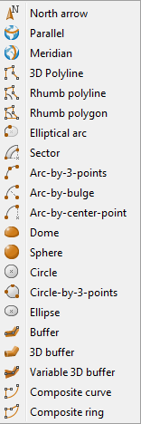
|
Clicking on a shape in the list while keeping the Shift-key pressed allows you to draw multiple shapes of the selected shape. A plus sign is added to the shape, and after you have drawn one shape, you can click on the map to draw another one. Click on the shape in the list again to disable this option. |
With the shape list you can quickly create one of the following shapes on the map. First select the shape in the list and then follow the drawing instructions for the selected shape:
Drawing North arrows
Use this shape to add a north indication to the map, as in Figure 66, “The north arrow”. Click on the map to indicate the location of the north indication.
To draw a North arrow on a 3D map, click the map once to set the location of the North arrow, and then click again to define the altitude of the arrow. The Object properties panel of a north arrow shows the following shape properties: location and altitude.
Drawing parallel lines
A parallel is a rhumbline (or loxodrome) with a constant latitude. Click on the map to indicate the start point of the parallel. Move the mouse and click again to indicate the end point of the parallel. You cannot add or remove points as a parallel always consists of two points. When you change one point, the other point changes automatically.
The Object properties panel of a parallel shows the following shape properties: a list with the two points of the parallel, the location and distance of the points, and the bearing to the next point.
Drawing meridian lines
A meridian is a rhumbline (or loxodrome) with a constant longitude. Click on the map to indicate the start point of the meridian. Move the mouse and click again to indicate the end point of the meridian. You cannot add or remove points as a meridian always consists of two points. When you change one point, the other point changes automatically.
The Object properties panel of a meridian shows the following shape properties: a list with the two points of the meridian, the location and distance of the points, and the bearing to the next point.
Drawing rhumb polylines
A rhumb polyline is a polyline that consists of rhumblines (or loxodromes). Click on the map to indicate the start point of the polyline. Move the mouse and click on the map to add extra points to the polyline. To add the end point to the polyline, double-click or right-click on the map.
The Object properties panel of a rhumb polyline shows the following shape properties: a list with the separate points of the polyline, the location of each point, and the bearing and distance to the next point.
Drawing 3D polylines
To create a 3D polyline, click on the map to indicate the start point of the polyline. Move the mouse and click on the map to add extra points to the polyline. To add the end point to the polyline, double-click or right-click on the map.
To create a 3D polyline on a 3D map, click on the map to indicate the start point of the map, then move your mouse to an appropriate altitude and click again to indicate the altitude of the first point. Each of the points on the polyline requires two clicks, one for position and one to mark the altitude. To add the end point to the polyline, double-click or right-click on the map.
The Object properties panel of a 3D polyline shows the following shape properties: a list with the individual points constituting the polyline, the location and altitude for each point, and the bearing and distance to the next point. If no terrain data is available, the altitude of a polyline point is 0 m by default.
Drawing rhumb polygons
A rhumb polygon is a polygon that consists of rhumblines (or loxodromes). Click on the map to indicate the start point of the polygon. Move the mouse and click on the map to add extra points to the polygon. To add the end point to the polygon, double-click or right-click on the map. The first point will automatically be connected to the last point to close the polygon.
The Object properties panel of a rhumb polygon shows the following shape properties: a list with the separate points of the polygon, the location of each point, and the bearing and distance to the next point.
Drawing elliptical arcs
Use this option to draw an elliptical arc on the map. Click on the map to indicate the center location of the arc. Move the mouse and click again to define the radius of the arc. The arc angle is $45^U+00B0$ by default and the A and B radii are equal. To change the radius of the arc, select one of the arc points and drag it to another location.
To draw an elliptical arc on a 3D map, click on the map to indicate the center location of the arc. Click two more times, once to define the A radius of the arc, and the second time to define the B radius. The next click defines the start position of the elliptical arc. Drag your mouse to draw the arc, and finish your arc by clicking again.
To change the rotation angle, select one of the end points of the A or B radius and move these on the map. It is also possible to enter exact values for the different angles and radii in the Object properties panel of the arc as described in Changing the shape properties. .
The Object properties panel of an arc shows the following shape properties:
-
The location of the start, center, and end point of the arc.
-
The angles of the start point (start angle) and end point (end angle), the difference between the start and end angle (arc angle), and the angle over which the arc is rotated (rotation angle).
-
The length of the A and B radius of the arc.
Drawing sectors or arcbands
Use this option to create a sector or an arcband. See Figure 67, “An example of a sector” and Figure 68, “An example of an arcband” for examples of these shapes. Click on the map to indicate the center location of the sector or arcband. Move the mouse and click again to define the radius of the sector or arcband. Next, move the mouse clockwise if you want to draw a sector, or counterclockwise if you want to draw an arcband. Also move the mouse up and down to define the size of the sector or arcband, and click once more to close the shape.
The Object properties panel of a sector shows the following shape properties:
-
The location of the center, the start and end points of the inner arcband, and the start and end point of the outer arcband.
-
The angles of the inner arcband (start angle) and outer arcband (end angle), the difference between the inner and outer arcband (arcband angle).
-
The length of the inner and outer radius.

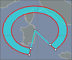
Drawing arcs-by-3-points
An arc-by-3-points is a circular arc defined by three points. Click on the map to indicate the start point of the arc. Move the mouse and click on the map to add the intermediate point to the arc. Finally, move the mouse and click on the map to add the end point to the arc.
The Object properties panel of an arc-by-3-points shows the following shape properties: the location of the start, intermediate, and end point.
Drawing arcs-by-bulge
An arc-by-bulge, as shown in Figure 69, “An example of an arc-by-bulge”, is a circular arc defined by a start and end point and a bulge. Click on the map to indicate the start point of the arc. Move the mouse and click on the map to add the end point to the arc. Finally, move the mouse and click on the map to define the direction of the bulge.
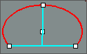
The Object properties panel of an arc-by-bulge shows the following shape properties: the location of the start and end point and the size and direction of the bulge. The sign of the bulge indicates whether the midpoint of the arc is on the left side (positive) or right side (negative) of the vector from the start to the end point. A bulge value of 1 means a half-circle, a value smaller than 1 means a less bulging arc and a value larger than 1 means an arc that bulges out in the start and end point.
Drawing arcs-by-center-points
An arc-by-center-points is a circular arc defined by a center point, radius, start angle, and arc angle. Click on the map to set the center location of the arc. Move the mouse and click on the map to set the radius and start angle of the arc (the start point). Move the mouse and click again on the map to set the arc angle (the end point).
The Object properties panel of an arc-by-center-points shows the following shape properties:
-
The location of the center, start, and end point of the arc
-
The angles of the start point (start angle) and end point (end angle) and the difference between the start and end angle (arc angle)
-
The length of the radius
Drawing domes
Click on the map to create the center location of the dome. Move the mouse and click again on the map to define the radius of the dome.
On a 3D map, click to create the center location of the dome. Move the mouse and click again on the map to define the radius of the dome. Finally, move the mouse up and down to determine an appropriate altitude for the base of the dome and click to finish drawing.
The Object properties panel of a dome shows the following shape properties: the location of the center point, the radius, and the altitude from the center (base altitude). The base altitude is 0 m by default if no terrain data is available.
|
It is also possible to select a sphere or circle and convert it into a dome by clicking on the Edit button and selecting the Convert into dome option. Enter the altitude of the base of the dome in the dialog box that pops up. |
Drawing spheres
Click on the map to create the center location of the sphere. Move the mouse and click again on the map to define the radius of the sphere. On a 3D map, click to create the center location of the sphere. Move the mouse and click again on the map to define the radius of the sphere. Finally, move the mouse up and down to determine an appropriate altitude for the center of the sphere, and click to finish drawing. The Object properties panel of a sphere shows the following shape properties: the location of the center point, the radius, and the altitude from the center (center altitude). By default the center altitude equals the radius so that it touches the ellipsoid.
|
It is also possible to select a dome or circle and convert it into a sphere by clicking on the Edit button and selecting the Convert into sphere option. Enter the altitude of the center point of the sphere in the dialog box that pops up. |
Drawing circles
Click on the map to indicate the center location of the circle. Move the mouse and click again on the map to define the radius of the circle.
The Object properties panel of a circle shows the following shape properties: the location of the center point and the radius of the circle.
Drawing circles-by-3-points
A circle-by-3-points is a circle defined by three points. Click on the map to indicate the first point of the circle. Move the mouse and click again on the map to define the second point of the circle. Repeat this step to add the third point to the circle.
The Object properties panel of a circle-by-3-points shows the following shape properties: the location of the first, second, and third point of the circle.
Drawing ellipses
Click on the map to indicate the center location of the ellipse. Move the mouse and click again on the map to determine the A and B radius of the ellipse. By default, the A and B radius have an equal length on a 2D map.
On a 3D map, the first click determines the center location of the ellipse, the second click determines the A radius, and a final third click determines the B radius. The Object properties panel of an ellipse shows the following shape properties:
-
The location of the center point.
-
The length of the A and B radius.
-
The angle over which the ellipse is rotated (rotation angle).
Drawing buffers
Click on the map to indicate the start point of the buffer. Move the mouse to determine the width and the shape of the buffer and click on the map to add extra points to the buffer. To add the end point to the buffer, double-click or right-click on the map.
On a 3D map, click on the map to indicate the start point of the buffer’s center line. To define extra center line points, make multiple clicks on the map. To add the end point to the buffer, double-click or right-click on the map. Then move the mouse to determine the width of the buffer, and finalize the drawing with one final click.
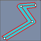
The Object properties panel of a buffer shows the following shape properties:
-
Buffer: a list with the separate points of the centerline of the buffer, the location of each point, and the distance and bearing to the next point.
-
Size: the width of the buffer and the style of the end cap of the buffer.
|
It is also possible to select a 3D polyline and convert it into a buffer by selecting the shape, clicking on the Edit button and selecting the Convert into buffer option. |
Drawing 3D buffers
Click on the map to indicate the start point of the 3D buffer. Move the mouse to determine the width and the shape of the 3D buffer and click on the map to add extra points to the 3D buffer. To add the end point to the 3D buffer, double-click or right-click on the map.
On a 3D map, click on the map to indicate the start point of the 3D buffer. Next, move the mouse up and down to determine the altitude of the start point, and click again. Each of the points on the buffer requires two clicks, one for position and one to mark the altitude. To finish the 3D buffer drawing, double-click to set the last buffer point.
The Object properties panel of a 3D buffer shows the following shape properties:
-
3D buffer: a list with the separate points of the centerline of the buffer, the location and altitude of each point, and the bearing and distance to the next point. The altitude of a point is 0 m if no terrain data is available.
-
Size: the width and height of the 3D buffer.
|
It is also possible to select a 3D polyline and convert it into a 3D buffer by clicking the Edit button and selecting the Convert into 3D buffer option. |
Drawing variable 3D buffers
Click on the map to indicate the start point of the variable 3D buffer. On a 3D map, move the mouse up and down to choose an altitude for the point, and click again. Move the mouse to determine the width and the shape of the 3D buffer and click on the map to add extra points to the variable 3D buffer. On a 3D map, you need to click once more to determine the altitude for each point. To add the end point to the variable 3D buffer, double-click or right-click on the map. After creating the buffer, the width of each point can be modified individually by moving the shape handles, or modifying the Object properties.
The Object properties panel of a variable 3D buffer shows the following shape properties: a list with the separate points of the centerline of the buffer, the location and altitude of each point, and the width, height below and height above properties of each point. The altitude of a point is 0 m, if no terrain data is available.
|
It is also possible to select a 3D polyline and convert it into a variable 3D buffer by clicking on the Edit button and selecting the Convert into variable 3D buffer option. |
Drawing composite curves
A composite curve is composed of multiple curves; each new curve starts where the previous curve ends. When you select the Composite curve from the shape list, an icon bar pops up in the top left corner of the map. It allows you to select the shape of the elements of the curve: polyline, rhumb polyline, arc-by-3-points, or arc-by-bulge. The last shape created before the selection of this shape is used by default. Click on the map to start the composite curve. Move the mouse and click on the map to add extra points to the composite curve. To add the end point to the composite curve, double-click or right-click on the map.
The Object properties panel of a composite curve shows a section for each element of the composite curve. This can either be polyline, rhumb polyline, arc-by-3-points, or arc-by-bulge. See the respective shape description for more information on the shape properties.
Drawing composite rings
A composite ring is composed of multiple curves. Each new curve starts where the previous curve ends and the last point of the last curve is connected to the first point of the first curve. When you select the Composite ring option, an icon bar pops up in the top left corner of the map. It allows you to select the shape of the elements of the ring: polyline, rhumb polyline, arc-by-3-points, or arc-by bulge. The last shape created before the selection of this shape is used by default. Click on the map to start the composite ring. Move the mouse and click on the map to add extra points to the composite ring. To add the end point to the composite ring, double-click or right-click on the map.
The Object properties panel of a composite ring shows a section for each element of the composite ring. This can either be polyline, rhumb polyline, arc-by-3-points, or arc-by-bulge. See the respective shape description for more information on the shape properties.
Shape actions
Once the shape is created it is possible to:
-
Select the shape: click on the shape. To select multiple shapes, keep the Shift-key pressed while selecting the shapes with the left mouse button. On a 2D map, you can click on the map, and keep the mouse button pressed while moving the mouse to draw a selection box that includes the shapes. When moving the mouse over a selected shape, the cursor shape changes to indicate that the shape is selected. When moving the mouse over a point of a selected shape, the cursor shape changes again to indicate that you can select the point to resize the shape or remove the point.
-
Move the shape to another location: select the shape and then drag and drop the shape to another location.
-
Resize the shape: select one of the points of the shape with the left mouse button and then drag the point to another location. On a 2D map, some shapes allow you to select the shape, press the Ctrl-key and drag the shape. An example of such a shape is a circle. The cursor shape changes to indicate that you can resize the shape.
-
Remove a point from the shape: press the Ctrl-key and select the point of the shape with the left mouse button to remove the point. The cursor shape changes to indicate that you can remove the point.
-
Add a point to the shape: press the Ctrl-key and select a location on (the edge of) the shape with the left mouse button to add the point.
-
Delete the shape: select the shape and press the Delete key. It is also possible to delete the selected shape by right-clicking and selecting the Delete option from the pop-up menu.
-
Insert a curve: to insert a curve in a composite curve or ring, select the shape, right-click and select the Insert curve menu item.
-
Copy (or cut) the shape and paste the shape as described in Copying and pasting objects.
|
Lucy allows you to copy shapes you created in a 2D map to a 3D map, and the other way around. To copy a shape, right-click the shape and select the Copy option from the menu. Then right-click in the other map, and select Paste from the menu. Lucy then copies the shape to the correct location on the map. |
Drawing options
After you have created one or more shapes, you can edit those shapes. To edit one or more shapes, select the shapes you want to change, and click the Edit button in the drawing toolbar. It offers the following drawing options:
-
Outline intersections: displays the intersection points of two or more shapes that overlap each other in the map view. This option is applicable to all types of shapes, even if they are on different layers, provided that they share the same georeference system.
-
Intersection: calculates and displays a new shape based on the intersection of two or more shapes that overlap each other in the map view. It supports points, polylines and polygons. Note that this option is only active if two or more supported shapes are selected.
-
Union: calculates and displays a new shape based on the union of two or more shapes in the map view. It supports points, polylines and polygons. Note that this option is only active if two or more supported shapes are selected.
-
Difference: calculates and displays a new shape based on the difference of two or more shapes in the map view. Typically the rightmost shape is subtracted from the leftmost shape. It supports points, polylines and polygons. Note that this option is only active if two or more supported shapes are selected.
-
Inverted difference: calculates and displays a new shape based on the difference of two or more shapes in the map view. Typically the leftmost shape is subtracted from the rightmost shape. It supports points, polylines and polygons. Note that this option is only active if two or more supported shapes are selected.
-
Symmetric difference: calculates and displays a new shape based on the symmetric difference of two or more shapes in the map view. It supports points, polylines and polygons. Note that this option is only active if two or more supported shapes are selected.
-
Convex hull: calculates and displays a new shape based on the convex hull of one or more shapes in the map view. It supports points, polylines and polygons. Note that this option is only active if one or more supported shapes are selected.
-
Make perpendicular: adjusts a polyline to make it perpendicular (or orthogonal) to another polyline. This option can only be used with polylines that only have a start and end point. Select the first polyline, click on the Edit button and select the Make perpendicular menu item. Finally select the second polyline. Note that due to the distortion of the projection, the lines may sometimes appear not to be orthogonal. This option is applicable to polylines on different layers, indifferent of their georeference system.
-
Extract offset line: creates a polyline parallel to another polyline. Select a polyline, click on the Edit button, and select the Extract offset line menu item. A dialog box appears in which you need to enter the distance between the lines and select to which side of the selected line the new polyline will appear. Note that this option is only applicable to one polyline.
-
Extract point: creates a point shape on a polyline. Select a polyline, click on the Edit button and select the Extract point menu item. A dialog box appears in which you need to enter the distance from the start or end point of the line. Note that this option is only applicable to one polyline. This option adds the default point shape to the polyline. For more information about changing the point shape, refer to Changing the shape style.
-
Convert into buffer: converts a 3D polyline or 3D buffer into a buffer. Select a 3D polyline or 3D buffer, click on the Edit button and select the Convert into buffer menu item. A dialog box appears in which you need to enter the width of the buffer and select the style of the end cap of the buffer. Note that this option is only applicable to one 3D polyline or 3D buffer.
-
Convert into 3D buffer: converts a 3D polyline into a 3D buffer. Select a 3D polyline, click on the Edit button and select the Convert into 3D buffer menu item. A dialog box appears in which you need to enter the width and the height of the 3D buffer. Note that this option is only applicable to one polyline.
-
Convert into variable 3D buffer: converts a 3D polyline into a variable 3D buffer. Select a 3D polyline, click on the Edit button, and select the Convert into variable 3D buffer menu item. Note that this option is only applicable to one polyline.
-
Extrude: extrudes a 2D shape into a 3D shape. Select one or more 2D shapes, click on the Edit button and select the Extrude menu item. A dialog box appears in which you need to enter the minimum and maximum altitude for the extruded shapes. If there is terrain data available, you can add the height of the terrain to the minimum and maximum altitudes by checking the ''Over terrain'' check box. Note that you cannot extrude the following shapes: north arrow, point, dome, and sphere.
-
Unextrude: converts one or more extruded shapes into a 2D shape.
-
Convert into dome: converts a sphere or a circle into a dome. Select one or more spheres or circles, click on the Edit button and select the Convert into dome option. Enter the altitude of the center point of the dome into the dialog box.
-
Convert into sphere: converts a dome or circle into a sphere. Select one or more domes or circles, click on the Edit button and select the Convert into sphere option. Enter the altitude of the center point of the sphere into the dialog box.
-
Delete: deletes the selected shape(s).
-
Group: groups two or more shapes. Grouped shapes are considered as one shape on which you can perform shape actions as described in Shape actions and drawing options that you can perform with the Edit button, provided that the action is applicable to more than one shape. For example you can move or duplicate grouped shapes but you cannot extract a point on a group of polylines.
-
Ungroup: ungroups a group of shapes.
-
Duplicate: duplicates one or more shapes. Note that the duplicated shapes are drawn at the same location as the original shapes so you need to move either the original or the duplicated shapes to see them both. When you have duplicated shapes, the duplicated shapes are automatically selected.
-
Translate: translates shapes over a certain distance and azimuth. Select one or more shapes, click on the Edit button and select the Translate menu item. Enter the distance and azimuth of the translation in the dialog box.
-
Copy style: copies the style information from a shape. Select the shape from which you want to copy the style, click on the Edit icon and select the Copy style menu item. The cursor changes into a cross, which indicates that you can use the left mouse button to select one or more shapes to which you want to copy the style. To select more than one shape on a 2D map, keep the Shift-key pressed.
Changing the shape properties
The Object properties panel of a shape allows you to view the shape properties and change the current values. By default, the Object properties panel appears in the top left corner of the application window after you have created a shape, but you can also open the panel by selecting a shape and double-clicking or right-clicking and selecting the Properties option. The Object properties panel only shows the properties of one selected shape. The contents of the Object properties panel change when you select another shape. When multiple shapes are selected, no object properties are shown. Figure 71, “The Object properties panel of a buffer” shows the Object properties panel of a buffer.
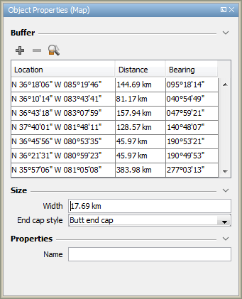
As Figure 71, “The Object properties panel of a buffer” shows, the Object properties panel consists of several sections. To expand a section, click on the section name or on the double arrow at the top of the section. Figure 71, “The Object properties panel of a buffer” shows the Object properties panel of a buffer with the Buffer section expanded. To collapse the section, click on the section name or on the double arrow at the top of the section.
The shape properties have the same units and formats as defined for the map and as described in Setting units, formats, and the coordinate system. To change a value, either enter a new value in the applicable text box or select a value from the drop-down list. The value
you enter in a text box is automatically validated. The background color of the text box will turn red if the entered value
is invalid. Click the left mouse button, or press the Enter key to make the new value effective. Press the Esc key to cancel
the last made change. The values for the different points of a shape are displayed in a list as shown in Figure 71, “The Object properties panel of a buffer”. To remove a point from the shape, select the point in the list and click on the Delete icon ![]() above the list. To add a point to the shape, select the point after which you want to insert the new point, and click on
the Insert icon
above the list. To add a point to the shape, select the point after which you want to insert the new point, and click on
the Insert icon ![]() above the list. If you did not select any point, the new point is added at the bottom of the list.
above the list. If you did not select any point, the new point is added at the bottom of the list.
Since each shape type has a specific set of properties, the Object properties panel of each shape type is different. Drawing shapes on the map describes the different shapes and their properties.
|
The Properties section shows the generic properties you defined at layer level while creating the drawing layer, as described in Adding a drawing layer. |
Changing the shape style
This section describes how to change the style of drawing shapes. Note that when you have selected one or more of drawing shapes on the map, the changes to the shape style only affect the selected shapes. If none of the objects are selected, the changes to the shape style will become the default for the next shapes you draw.
Depending on the shapes that were selected, the drawing toolbar allows you to change one or more of the following shape styles:
-
 The line color and transparency, as described in The color selector.
-
 The fill color. A menu pops up that allows you to select No Fill or Choose Fill Color. If you select Choose Fill Color, a dialog box allows you to change the fill color and transparency, as described in The color selector.
-
 The line thickness.
-
 The line style. Figure 72, “The line style options” shows the possible style options.
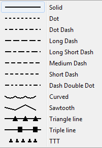 Figure 72. The line style options
 -
 The arrow shape. A menu pops up which allows you to choose if lines should have an arrow at the begin, end, or at both sides.
Select No Arrow to remove the arrows from the line.
The arrow shape. A menu pops up which allows you to choose if lines should have an arrow at the begin, end, or at both sides.
Select No Arrow to remove the arrows from the line.
-
 The point icon. A dialog box appears from which you can select a figure to represent points on the map. Figure 73, “The point shapes” shows the dialog box with point shapes.
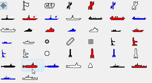 Figure 73. The point shapes
It is also possible to copy the style from another shape by selecting the Copy style option, as described in Drawing options.
To change the font settings, click on the Font icon![]() next to the color and style icons. A dialog box allows you to set the following text characteristics:
next to the color and style icons. A dialog box allows you to set the following text characteristics:
-
Font: the box shows the current font. You can select another font from the font list.
-
Effects: select the appropriate check boxes to make the text bold or italic.
-
Color: to change the text color, click the dotted button to open the color selector and select text color and transparency, as described in The color selector.
The Preview in the dialog box shows sample text with the selected settings.
To change the text, select the text on the map, right-click and select Properties from the pop-up menu. Enter the new text in the Text box of the Properties panel.
|
When you select a shape other than a drawing shape, such as a flight trajectory for example, the style options on the drawing toolbar are not available. |
Loading and saving drawing layers
Lucy supports the following file formats for loading and saving drawing data:
-
.drawing: LuciadLightspeed’s default file format for storing drawing data.
-
.shp: Note that a .shp file can only contain one object type: either points, polylines, or polygons. Style information, such as colors, is not supported.
-
.mif: Note that a .mif file can only contain points, polylines, polygons, rectangles, arcs, ellipses, and text. Style information is stored partially: only colors and line widths are stored.
-
.pol: Note that a .pol file can only contain polylines and polygons. Style information such as colors, is not supported.
-
.red: LuciadLightspeed’s formerly used file format for storing drawing data. Note that it is only possible to load data from .red files and not to save drawing data to .red files.
To load drawing data, you can:
-
Select the File→ Open menu item. A dialog box allows you to load .drawing files and import .red files as .drawing files. Note that although the dialog allows you to load .shp, .mif, and .pol files, these files are not imported as .drawing files. Only for the loaded .drawing and .red files, a corresponding drawing layer that allows you to create layers is added to the layer tree.
-
Click on the Load drawing data icon
in the drawing toolbar. A dialog box allows you to load .drawing files and import .shp, .mif, .pol or .red files as .drawing
files. The loaded file appears in the layer tree as a drawing layer in which you can create shapes. Note that although the
drawing functionality for the imported .shp, .mif, and .pol files is the same as for other drawing files, the properties of
the loaded data differ from Lucy’s shape properties. Some information might be lost.
- Map-centric Lucy
-
To import drawing files in map-centric Lucy, go to Data → Import as drawing….
To save a selected layer to a .drawing file, click on the Save current layer icon ![]() in the drawing toolbar. A dialog box allows you to specify the name and the location of the .drawing file. Note that when
you save a .shp, .mif, or .pol file to a .drawing file and then load the .drawing file, the properties of the originally loaded
data differ from Lucy’s shape properties. You can also use the File→ Save As menu item to save a drawing layer to a .drawing file.
in the drawing toolbar. A dialog box allows you to specify the name and the location of the .drawing file. Note that when
you save a .shp, .mif, or .pol file to a .drawing file and then load the .drawing file, the properties of the originally loaded
data differ from Lucy’s shape properties. You can also use the File→ Save As menu item to save a drawing layer to a .drawing file.
When you save a workspace that contains drawing data, the drawing data is stored in a separate .drawing file. Loading and saving workspaces provides more information on loading and saving workspaces. For more information on working with layers, refer to Working with layers.
Exporting drawing layers
To export a selected drawing layer to a .shp, .mif, or .pol file, click on the Save current layer icon ![]() in the drawing toolbar. A dialog box allows you to specify the name and the location of the file. Select the file type from
the Files of type drop-down list. Note that when you export a drawing layer to another file format the restrictions mentioned in the list of
supported file formats above apply here as well. It is possible that some information is lost.
in the drawing toolbar. A dialog box allows you to specify the name and the location of the file. Select the file type from
the Files of type drop-down list. Note that when you export a drawing layer to another file format the restrictions mentioned in the list of
supported file formats above apply here as well. It is possible that some information is lost.
- Map-centric Lucy
-
To export a drawing layer in map-centric Lucy, go to Data → Export drawing as….
Displaying your data in other view types
Map data cannot only be displayed in a 2D and 3D map. It is possible to display map data in other views that offer additional functionality. This article describes the Map Overview panel and the additional views that Lucy offers to display map data. Extended functionality describes which views are added by installing extra LuciadLightspeed components.
Getting a map overview (Lucy GXY)
By default, the panel with the map overview is displayed top left of the Map panel. If the panel is closed you can open it by selecting the Tools→ Map Overview menu item.
The main purpose of the map overview is to give an outline of the displayed map(s) but it also allows you to navigate around a map quickly by editing the map outline. Figure 74, “The default Map Overview panel” shows the default Map Overview panel.
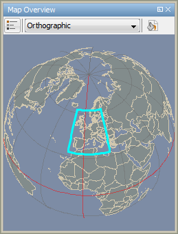
The cyan rectangle in the Map Overview panel represents the area of the map that is visible in the map view. You can move the displayed area in the map view by dragging the rectangle in the Map Overview panel or you can change the displayed area in the map view by resizing the rectangle. To create a new area to display click outside the current outline in the Map Overview panel and drag the mouse to draw a new outline. When multiple maps are opened you can click on an outline to see the name of the corresponding map.
The title bar of the Map Overview panel contains the same icons as the Map panel and the Map Layers panel as described in Rearranging panels. Additionally the Close icon allows you to close the panel. The toolbar of the Map Overview panel contains the following box and icons:
-
The Projection box shows the currently active projection of the Map Overview. To change the projection, select one of the options of the drop-down list as described in Changing the map projection. Note that the projection of the Map Overview may differ from the projection of the map in the map view.
-
The Change map background color
 icon opens the color selector which allows you to select another color for the background of the map overview as described
in The color selector.
icon opens the color selector which allows you to select another color for the background of the map overview as described
in The color selector.
Displaying your data in a table view
The table view shows the objects of a selected layer and their properties in table format. To open the table view first select one or more layers in the layer tree and either:
-
Press Ctrl+t.
-
Select the File→ New→ Table View menu item.
-
Right-click in the layer tree and select Table View from the menu that appears.
A separate panel appears, by default under the map view, for each of the selected layers, and the first 1000 elements of the layer source data are displayed in rows.
If a layer has no objects, the Table view menu items are grayed out. Figure 75, “The table view of a countries layer located under the map view” shows the table view of the world layer.
- Map-centric Lucy
-
To view layer data in a table in map-centric Lucy, select the layer, and click the Table icon in the lower left corner of the side tool bar. To close the view, click the Table icon again.
|
Note that when you select another layer or when you switch to another map, the table contents adapt to the newly selected
layer. To lock the table contents for the currently selected layer, click on the Automatically lock on the current layer |
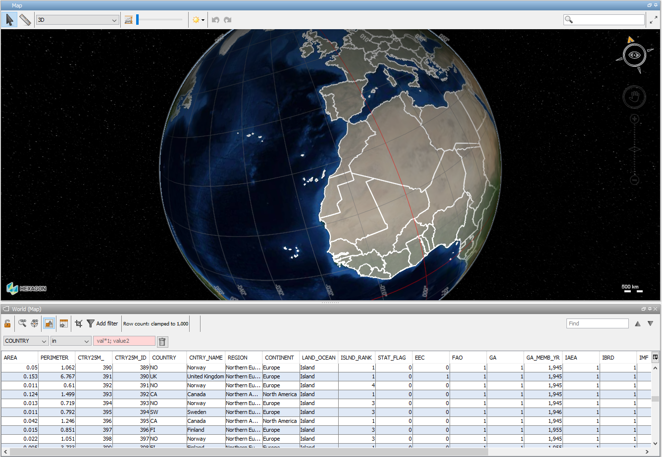
Whenever the table view is in the process of searching the layer source data, the busy icon ![]() next to the Row count indicates that not all data for that layer has been loaded yet.
next to the Row count indicates that not all data for that layer has been loaded yet.
Searching the data in the table
You can search the data displayed in the table by entering a search term in the Find field at the top right of the table. To move the focus from the table to the search field, Press Ctrl+F. All object properties in the table are searched for a match. The Up and Down arrows next to the field allow you to scroll through the search results in the table.
|
To search the complete layer data source, and not just the data elements present in the table, use the Lucy search field in the map tool bar. |
Restricting the table content to visible data
To restrict the items in your table to just the objects visible in the map view, click the Only show elements visible on map  icon.
icon.
While the icon is selected, the table content adapts as the user pans or zooms in the map view.
Filtering the layer data from the table view
To configure a filter for the table view and the layer data shown in the map view, click the Add filter  icon.
icon.
|
The table data may already have been filtered in some way, through the presence of a companion styling and filtering file, for example. In that case, the Add filter icon is disabled. |
A filtering tool bar is added to the table view. It allows you to configure the filter:
-
Select the column containing the values you want to filter on in the first drop-down menu.
-
Select a filter operator in the second drop-down menu. The operator options change depending on the value type of the column selected in the first drop-down menu.
-
Enter a selection value in the third filter field. The value format depends on the filter operator selected in the second drop-down menu. In some cases, the field provides hints on the format you can apply to the selection.
-
Press ENTER to see the filter results. The table view row count will be updated based on the number of results returned.
To start over with your filter configuration, click the Delete icon next to the filter fields.
Changing the table column display
The Visibility icon ![]() at the right of the last column allows you to change the display of the columns in the table view. Click on the icon to display
the list of columns. Select a column to show it in the table and deselect the column to hide it. If the option Horizontal Scroll is selected, the columns are sized to their contents and a horizontal scroll bar appears under the table to scroll through
the columns. If this option is not selected, all columns are resized to fit in the available table width. Select the menu
item Pack All Columns or Pack Selected Columns to fit all or the selected columns to their contents.
at the right of the last column allows you to change the display of the columns in the table view. Click on the icon to display
the list of columns. Select a column to show it in the table and deselect the column to hide it. If the option Horizontal Scroll is selected, the columns are sized to their contents and a horizontal scroll bar appears under the table to scroll through
the columns. If this option is not selected, all columns are resized to fit in the available table width. Select the menu
item Pack All Columns or Pack Selected Columns to fit all or the selected columns to their contents.
Sorting the data
Clicking on the column header sorts the column data in ascending order. First, the data currently loaded in the table view is sorted, quickly followed by a sorting of the source of the layer data, and an update of the table view with the first 1000 sorted elements.
Clicking again on the column header sorts the column data in descending order. Click a third time on the column header to undo the sorting of the column data.
Selecting table items and adjusting the map view
Select one or more objects (rows) in the table and adjust the map view to the selection by using one of the icons above the table:
-
 Automatically fits the map view to the selected objects. If the table selection changes, the map view will automatically
fit to the new selection. If this option is enabled, the Auto center option is disabled.
Automatically fits the map view to the selected objects. If the table selection changes, the map view will automatically
fit to the new selection. If this option is enabled, the Auto center option is disabled.
-
 Automatically centers the selected objects in the map view. If the table selection changes, the center of the map view will
automatically change to the new selection without zooming. If this option is enabled, the Auto fit option is disabled.
Automatically centers the selected objects in the map view. If the table selection changes, the center of the map view will
automatically change to the new selection without zooming. If this option is enabled, the Auto fit option is disabled.
-
 Automatically selects the selected objects in the map view. If the selection in the table changes, the selection in the
map view will automatically change. Note that if the selection in the map view changes, the selection in the table will automatically
change, irrespective if this option is enabled or not.
Automatically selects the selected objects in the map view. If the selection in the table changes, the selection in the
map view will automatically change. Note that if the selection in the map view changes, the selection in the table will automatically
change, irrespective if this option is enabled or not.
When you right-click a table row, a menu allows you to perform the following actions on the selected objects:
-
Copy the selected items. Select this option (or use Ctrl+C) to copy the selected data to another file format, for example a database or spreadsheet. Use Ctrl+A to select all data.
-
Fit map and select the selected items. The map fits to the selected objects and the objects are selected in the map view. You can also press Enter to do this.
-
Center map and select to the selected items. The map is centered to the objects, and the objects are selected in the map view. Note that the Auto center icon above the table automatically centers the map to the selected items.
-
Delete the selected items. The selected data objects are removed from the table, the map view, and the data set.
|
You can delete data objects from the table only if the data belongs to an editable layer. For more information, see The layer tools and options. |
Exporting the table data to a file
To export the table data to a file, select the data in the table, and click the ![]() icon.
icon.
The selected data is saved to a .csv file. A dialog box appears in which you can browse for an existing file or enter the name of a new file.
Only data present in the table view is exported, so 1000 data elements are exported at most.
Comparing object properties
Lucy allows you to compare the properties of multiple objects by displaying their object properties panels next to each other in a comparison view. The comparison view shows the properties of selected objects alongside each other. To open the comparison view, select Tools | Compare Objects.
To compare objects in the comparison view:
-
Select at least one object. To select multiple objects, press Shift.
-
Right-click the selected objects on the map, and select Compare from the options menu. If it was not open yet, the comparison view panel opens below the map view. It displays the object properties panels for the selected objects side-by-side, with a maximum of 4 panels.
Figure 76, “The comparison view of two AIXM objects located below the map view” shows a comparison view for two AIXM taxiway element objects.
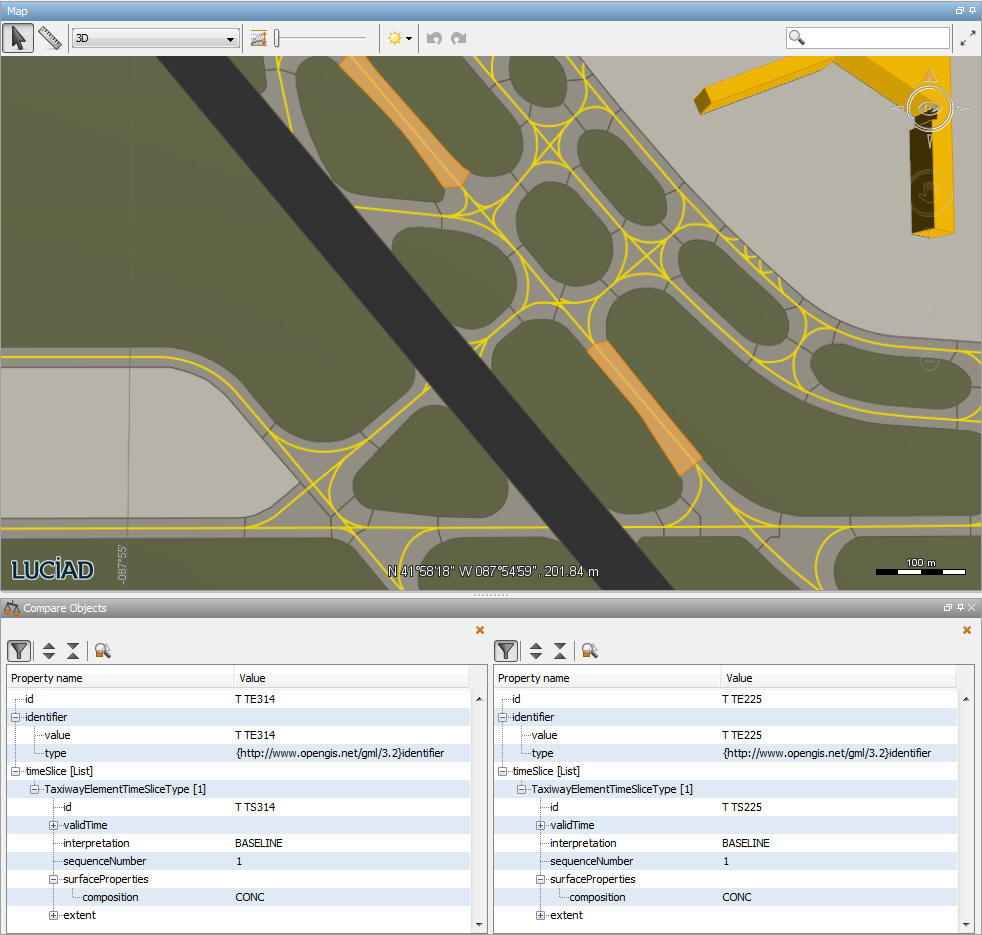
|
You can select any vector object for addition to the comparison view, as long as it is in a layer that is selectable. To learn how to make a layer selectable, see The layer tools and options. You can select objects from distinct layers for comparison. |
Use the same steps to add more objects to the comparison view. There is a limit on the number of objects you can compare to each other, though. If you add more objects, Lucy closes the properties panels of the first objects in the comparison view.
To prevent Lucy from closing panels that you still need, you can make room up front by closing the panels you no longer need.
To remove an object from the comparison view, simply close its properties panel by clicking the  icon .
Displaying shape height in a vertical view
The vertical view is a panel that displays a map line, polyline or buffer in a height graph. To open the vertical view, select the File→ New→ Vertical View menu item. The panel for the vertical view appears below the map view.
To display a line or buffer vertically, select it on the map. The vertical view updates automatically when changes are made to the line on the map, or when another map or shape is selected.
Figure 77, “Terrain data in the vertical view” shows the vertical view with terrain data.
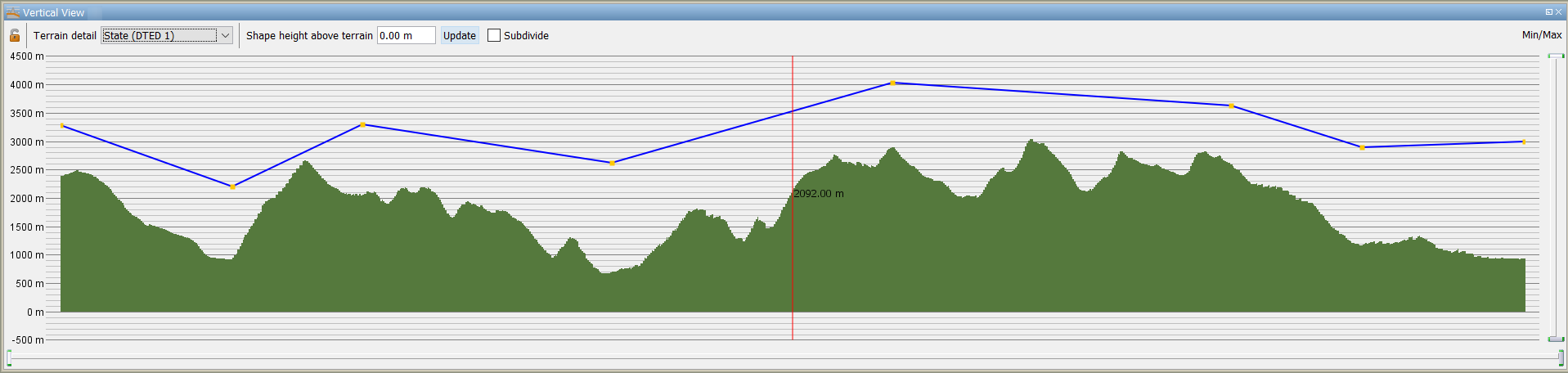
|
Make sure to load elevation data as well, if you want to see the selected line displayed in relation to terrain height. |
- Map-centric Lucy
-
To display a line or buffer in a height graph in map-centric Lucy, select the line, and click the Profile view icon in the lower left corner of the side tool bar. To close the view, click the Profile view icon again.
The vertical view allows you to select a DTED level in the Terrain detail dropdown menu. The DTED level determines the terrain resolution in the vertical view. See [DTED_level] for more information.
Zooming in on shape sections or height ranges
To limit the view to particular line sections or to a particular height, use the sliders next to and below the line to view sections of the line.
To set the minimum and maximum display height, use the Min/Max button above the line. This allows you to zoom in or out on specific sections of the view.
Changing the height of the shape
To change the height of the selected shape, either drag one or more points of the shape in the vertical view to the required altitude.
Alternatively, select the points in the Object properties panel and enter the desired height in the Altitude column. To open the Object properties panel at the top left of the map view, double-click on the line in the map view .
Move the entire shape above the terrain
To make sure that the shape is above the terrain:
-
Enter the required height of the line above the terrain in the Shape height above terrain field.
-
If you want to add extra points in between the shape points to make sure that the entire shape is at the required height above the terrain, select the Subdivide check box
-
Click Update.
The altitudes in the Object properties panel of the line are automatically updated.
Displaying a compass grid in the radar view (Lucy GXY)
The default radar view allows you to add a compass grid around a selected object in the map view showing the direction to other objects on the map. To display the compass grid, select the Tools→ Radar View→ Compass grid menu item. Figure 78, “A compass grid around Paris” shows a compass grid around Paris.
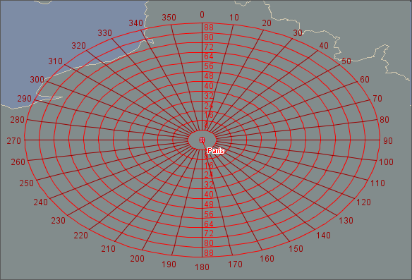
When a moving object is added to the map, it is possible to link a camera to the moving object and follow the object while moving as described in [linking_camera]. The compass grid changes according to the selected camera option.
Terrain
Lucy allows you to load and display the following terrain data in 2D:
-
Terrain (
.trn) files that are created with the 3D Terrain wizard from earlier versions of Lucy. -
Earth terrain repositories (
tilerepository.cfg) that are created outside Lucy, or with the 2D Terrain wizard from earlier versions of Lucy, or with the Export as Earth repository menu item as described in Saving a terrain to a repository (Lucy GXY).
Working with terrain repositories
A terrain repository consists of a tile set that is saved with a fixed resolution. Lucy uses a hierarchical tiling mechanism to display tile sets for the selected display area in the view. Only the tiles of the selected area are displayed, which has huge performance gains when rendering large terrains.
Loading a terrain repository
To load a terrain repository, select the File→ Open menu item. A dialog box appears in which you can specify the location of tilerepository.cfg. The repository is added as a separate layer to the layer tree with the name of the folder from which it is loaded. Note
that the layer structure of the source data is not maintained as the repository contains one tile set. When zooming in on
a specific area of the loaded terrain it may take some time before the selected tile sets are displayed in the proper resolution
as explained in Working with terrain repositories.
|
When loading a terrain repository created with an earlier version of Lucy or LuciadLightspeed, the loading may take longer than loading new terrain repositories because the tile sets are matched to the current tile set definition. |
Saving a terrain to a repository (Lucy GXY)
It is not only possible to load and display terrain data but also to save a combination of one or more of the following files to a terrain repository:
-
.trn files
-
tilerepository.cfg files
-
raster files
|
You can only use the Export to earth repository functionality in Lucy GXY. |
Use the File→ Export to Earth repository menu item to save loaded data to a terrain repository. A dialog box appears as shown in Figure 79, “The dialog box for saving a terrain to a repository” which allows you to select an empty directory in which you can save the repository and specify the repository settings. Note that when loading the repository, the directory name is used as name for the corresponding layer.
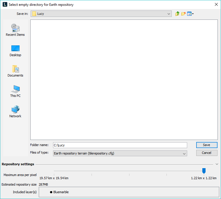
The repository saves all visible layers with terrain and/or raster data to one tile set. If you do not want to include layers in the repository you can hide those layers as described in The layer tree popup menu. Use the slider in the Repository settings section to define the resolution of the terrain. The size of the repository depends on the defined resolution and the estimated size is displayed under the slider. The higher the resolution, the bigger the repository and the longer it takes to create the repository. Keep an eye on the estimated repository size and adjust the resolution to ensure a reasonable repository size.
Click on the Save button to save the repository as tilerepository.cfg. A dialog box appears that shows the progress of preprocessing the data as shown in Figure 80, “The dialog box for preprocessing a terrain”. The preprocessing may take a few minutes for small terrains and for multi-leveled raster data as the tiles for the most
detailed level are processed first. Once the first level is created, the processing of the tile sets for the other levels
is much faster. During the preprocessing of the data you cannot use Lucy’s user interface. Close the dialog box when all data
is processed.
|
Consider the size of the data you want to store in a terrain repository before you start the saving process. It is advisable to use Lucy only for saving relatively small terrains to a repository. If you are dealing with tens of gigabytes, you may want to dedicate a computer to the storage process for a while. If you need to handle extremely large terrains, detailed worldwide data that amounts to hundreds of gigabytes for example, consider using an alternative solution that is designed specifically for this purpose, such as the LuciadFusion product. |
Printing and exporting maps
This article describes the options for printing a map or defined area on a map, and exporting a map to an image.
Printing a map
You can print the entire map displayed on your screen, or you can select an area of the map and only print that area. For more information about selecting a print area, see Defining a print area.
You can also choose to print the map on one page, or spread it across more pages. If you decide to print on one page, the map will be fitted to exactly one printed page. If you are printing on more pages, you can define over how many pages you want to spread the map. To learn more about these print settings, see Viewing and editing the print settings. For more information about page settings, refer to Defining the page setup. Before printing, you can preview the map print on screen by selecting the File→ Print Preview menu item, and select new settings if needed. Printing the map describes how to print the map.
Defining a print area
If you want to print a specific area of a 2D map in Lucy GXY, rather than the entire map displayed on screen, you can select a print area. To define a print area on a map, select the File→ Define Print Area menu item. Click on the map to start drawing the area and move the mouse to define the area. Click once more to finish the creation of the area. The resulting rectangle contains the map area that will appear on your print-out, as well as a well as shaded section that indicates how much space of your printout will be covered by a page footer with extra information. To learn more about defining the information in this footer, see Viewing and editing the print settings.
To resize the print area, move the mouse over one of the corners of the area until the cursor shape changes. Click with the left mouse button and drag the corner to resize the area. The width and height will change relative to each other to keep the aspect ratio and avoid distortion of the map. To move the area, move the mouse over the area borders until the cursor shape changes. Click with the left mouse button and drag the area to another location.
|
You can only define one print area on the map. As soon as you select the File→ Define Print Area menu item, a previously selected print area is removed. |
When you have defined a print area, a Print Area layer is added to the layer tree and a Print Area panel displaying properties for the print area opens at the top left of the map view, as shown in Figure 81, “The Object properties panel of a print area”. In the Object properties panel you can define some of the print settings as described in Viewing and editing the print settings. The selected print area automatically adjusts to your new settings.
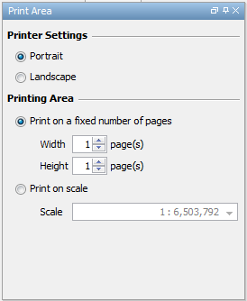
Use the Printer Settings options Portrait and Landscape to change the paper orientation of your printout.
The Print on a fixed number of pages option allows you to change the number of pages on which the map is printed . This is useful to spread larger maps across more printed pages. To expand the print area horizontally over more pages, increase the number of pages in the Width spin box. To expand the print area vertically over more pages, increase the number of pages in the Height spin box. Figure 82, “A landscape print area with a height of two pages and a width of two pages” shows a print area on the map that will be printed on four pages in landscape. The Width and Height spin boxes have both been set to 2.
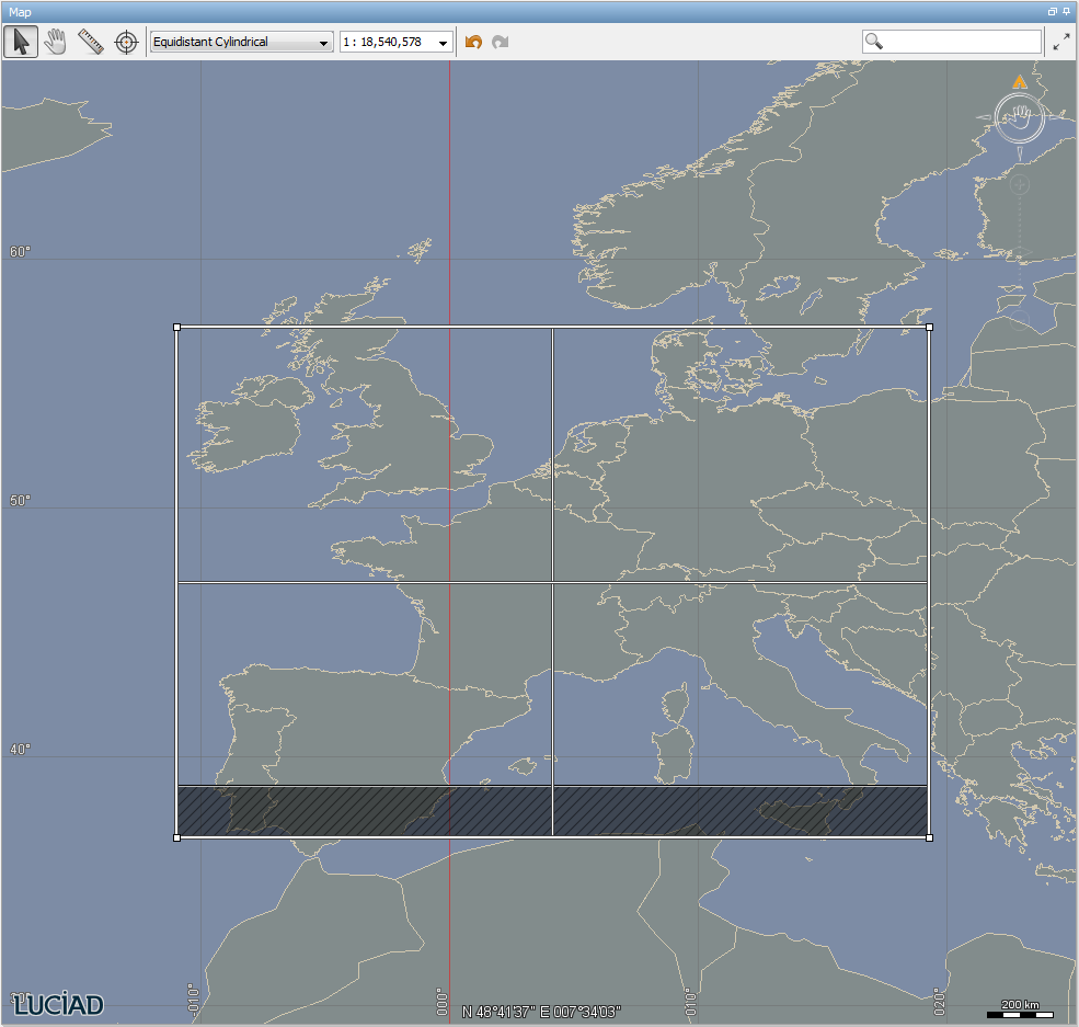
You can also indicate a scale to print the map area on, instead of specifying an exact number of pages. The Print on scale option allows you to select a specific scale from the Scale dropdown menu. In that case, Lucy will calculate the number of pages required to print the map.
If you want more print options than the ones displayed on the Print Area panel, open the menu{Print preview} page. For more information about these options, see Viewing and editing the print settings.
Viewing and editing the print settings
You can view and change printing options from the Print Preview window. Open the Print Preview window by selecting the File→ Print Preview menu item. The Print Preview window contains the following sections in which you can view and edit the print settings. The preview area will automatically adjust to new settings. Figure 83, “The Print Preview page” shows the Print Preview window.
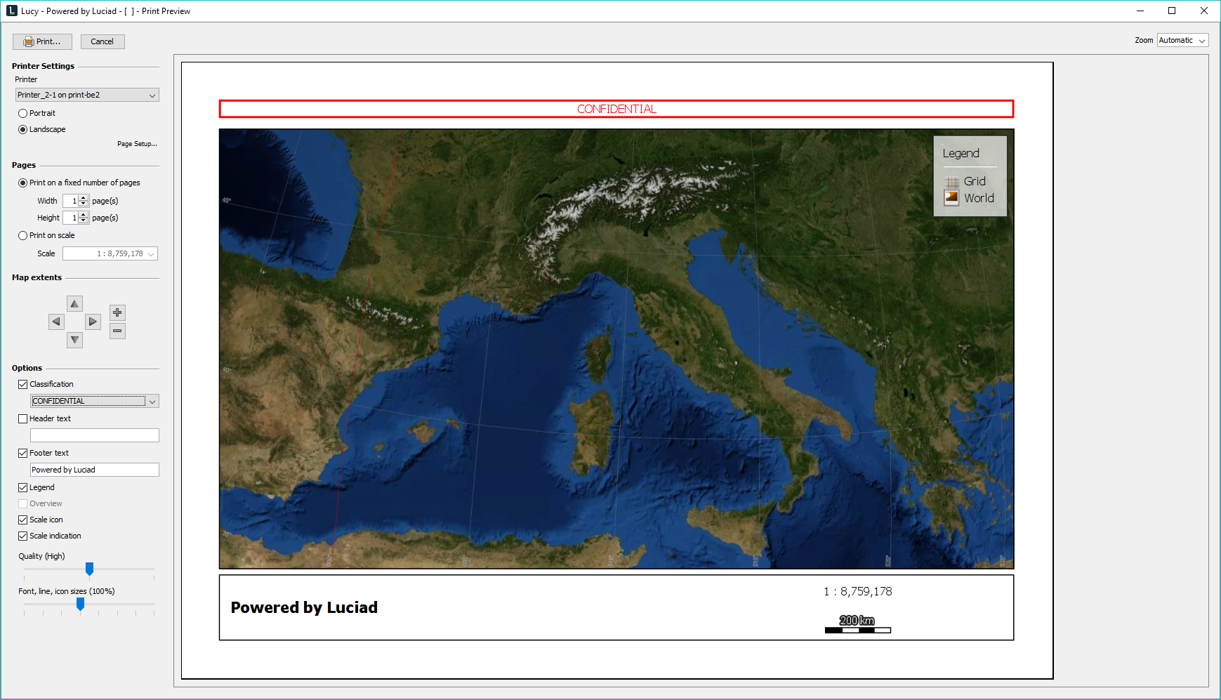
-
Printer Settings
-
Printer: to define the printer. The default printer as defined in the print settings of the operating system is selected by default, use the drop-down list to select another printer.
-
Paper orientation: select Portrait to fit the map to a vertically oriented page, or Landscape to fit the map to a horizontally oriented page. This setting corresponds to the the Orientation page setting described in Defining the page setup.
-
Page Setup: to open the Page setup dialog box as described in Defining the page setup.
-
-
Pages
-
Print on a fixed number of pages: allows you to change the number of pages on which the map is printed . This is useful to spread larger maps across more printed pages. To expand the print area horizontally over more pages, increase the number of pages in the Width spin box. To expand the print area vertically over more pages, increase the number of pages in the Height spin box. The map printing scale will automatically be calculated.
-
Scale allows you to select a specific print scale from the Scale dropdown menu. Lucy will calculate the number of pages required to print the map at the selected scale.
-
|
If you select a large print scale, Lucy will request your confirmation before generating a preview, because this might take a long time. Click the Generate Preview button if you want to create a preview regardless of the time it takes. |
-
Map extents: click the arrow buttons to shift the visible map area in the preview up and down, or to the left and right. Click + or - to zoom in or out on the map in the preview.
-
Options
-
Classification: to indicate an information classification at the top of the page, as shown in the preview area. You can select a classification level from the drop-down menu below.
-
Header text: to include page header text, as show in the preview area. You can add a header text in the text box below.
-
Footer text: to include a page footer text, as shown in the preview area. You can change the footer text in the text box below.
-
Legend: to include the legend as shown in the preview area.
-
Overview: to include the Overview map in the page footer.
-
Scale icon: to include the scale icon in the page footer.
-
Scale indication: to include the scale indication in the page footer.
-
Quality: to define the print resolution. Use the slider to adjust the quality of your printout.
-
Font, line, icon sizes: to define the ratio of the pixels on screen to the pixels on paper. A higher value results in wider lines, larger fonts and icons.
-
-
Print button: opens the Print dialog box to print the map as shown in the preview area.
-
Cancel button: closes the Print Preview page without printing.
-
Zoom dropdown menu: determines the scale of the preview. Use the drop-down list to select another scale. Use a small scale when viewing a map that is spread across multiple pages.
- Map-centric Lucy
-
To view and edit print settings in map-centric Lucy, go to Data → Print preview….
Defining the page setup
To define the page setup and additional printer settings, click the Page Setup link in the Print Preview window. The File→ Page Setup menu item offers the possibility to define printer settings. Which printer settings are available depends on the operating system.
-
Paper: the paper size and paper source, depending on the selected printer.
-
Orientation: Portrait to print vertically on the page, or Landscape to print horizontally on the page. This setting is the same as the Paper orientation described in Viewing and editing the print settings.
-
Margins: the print margins
-
Printer: the printer and the printer properties. Refer to the printer settings of your system.
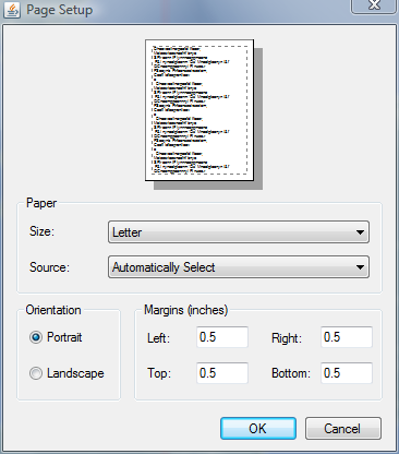
Printing the map
To print the entire map or a defined print area, select the File→ Print menu item or the Print button in the Print Preview window. The Print dialog box allows you to select a printer, define its properties, define the pages and the number of copies to print.
|
If a print area has been defined and its layer is visible, the print area is printed. If no area is defined, the current map boundaries are used for printing. |
- Map-centric Lucy
-
To print the map in map-centric Lucy, go to Data → Print…, or click Print in the Print Preview window.
Exporting the map to an image
To save the map as an image, select the File→ Save As Image menu item. A dialog box pops up that allows you to choose the format, the name, and the location of the image file. By default the following image file formats are supported: GIF, JPEG, and PNG files. Exporting to a GeoTIFF map saving format is supported by Lucy GXY only.
For the following file formats you can specify additional settings:
-
JPEG: the quality of the encoded image (where 1 is the best quality)
-
GeoTIFF (Lucy GXY):
-
Compression: compress the file without data loss (lossless) or with some data loss (JPEG lossy) or do not compress the file
-
Level count: the number of raster levels that vary in detail and that should be computed on the fly and saved to the GeoTIFF file. When selecting Keep original, the original levels of the input raster are encoded. When selecting a value of 1 or higher, the additional levels of detail are computed and encoded.
-
Quality: the quality of the encoded image (where 1 is the best quality)
-
Scale factor: the factor between the levels
-
Tile height: the height of a tile in pixels
-
Tile width: the width of a tile in pixels
-
|
Note that the resolution of the saved image will be the same as the number of pixels in the map view. This implies that even when a high-resolution raster format is visible in the map view, the image resolution will be limited to the number of pixels in the map view. |
Extended functionality
Extended Lucy functionality
There are number of additional LuciadLightspeed components that extend the default functionality offered by Lucy. Lucy also supports many more data formats in addition to the default data formats. These additional data formats require the installation of the corresponding components as well.
Table 3, “Supported data formats” in Appendix A, Supported data formats indicates which data formats you can use in Lucy after installing the corresponding component. Refer to Appendix B, Acronyms and abbreviations for definitions of the acronyms and abbreviations.
This part describes the available components and their extended functionality and format support.
After installing a component for the support of an additional data format, you can load files in the corresponding data format by using the File→ Open menu. You can select the additional data format from the Files of type drop-down list in the dialog box that appears. When the data is loaded, a layer is added to the layer tree.
- Map-centric Lucy
-
To load files in map-centric Lucy, go to Data → Open…. To connect to services, go to Data → Connect to…. To view and edit object properties from map-centric Lucy in a properties panel , just click the object on the map. Map-centric Lucy automatically displays a previewer for data with a time component.
Advanced Raster Connectors
After installing the Advanced Raster Connectors component, you can load a number of additional raster formats. See Appendix A, Supported data formats for more detail.
Database Connectors
After installing the Database Connectors component, you can load SQL Server, Oracle, and PostgreSQL PostGIS data formats.
The Microsoft SQL Server component
The Microsoft SQL Server component adds support for loading vectorial data from an Microsoft SQL Server file . Loading this type of data requires a .mss file which contains the properties of the data to load. See the SQL Server documentation for more information about the .mss file format.
The Oracle GeoRaster component
The Oracle GeoRaster component adds support for loading raster data from an Oracle Spatial database. Note that loading this type of data requires an .ogr file which contains the properties of the data to load. See the Oracle Spatial documentation for more information about the .ogr file format.
The Oracle Locator component
The Oracle Locator component adds support for loading vectorial data from an Oracle Locator or Spatial database. Note that loading this type of data requires an .ora file which contains the properties of the data to load. See the Oracle Locator documentation for more information about the .ora file format.
The PostgreSQL PostGIS component
The PostgreSQL PostGIS component adds support for loading 2D and 3D vector data from a PostgreSQL database that has been spatially enabled with PostGIS. Note that loading this type of data requires a .pgs file with the properties of the data. See the PostgreSQL PostGIS documentation for more information about the .pgs file format.
The Terrain Analysis Engine
After installing the Terrain Analysis Engine component, you can perform additional hypsometric analysis on the elevation data you have loaded in Lucy.
For some functionality, such as the calculation of elevation contours, you must use Lucy GXY.
Apply hypsometric analysis to your elevation data layer
|
The information in this section applies to Lucy and Map-centric Lucy maps only. To learn about the hypsometry functionality in Lucy GXY, see Using the Terrain Analysis Engine in Lucy GXY. |
You can add map layers that apply height-related calculations to elevation data, and present the results by applying a specific color range to the elevation data.
-
Hypsometric shading. Manipulate the direction and angle of inclination of sunlight to calculate and visualize shading on the terrain.
-
Azimuth. Visualize the azimuth of points on the terrain with reference to a direction that you can change on the azimuth layer properties.
-
Orientation. Compute and visualize the angles of steepest descent of the terrain with reference to a given direction.
-
Slope. Compute and visualize slope rate in a range of colors.
-
Ridges and valleys. Calculate and visualize in color where the ridges and the valleys are on a terrain.
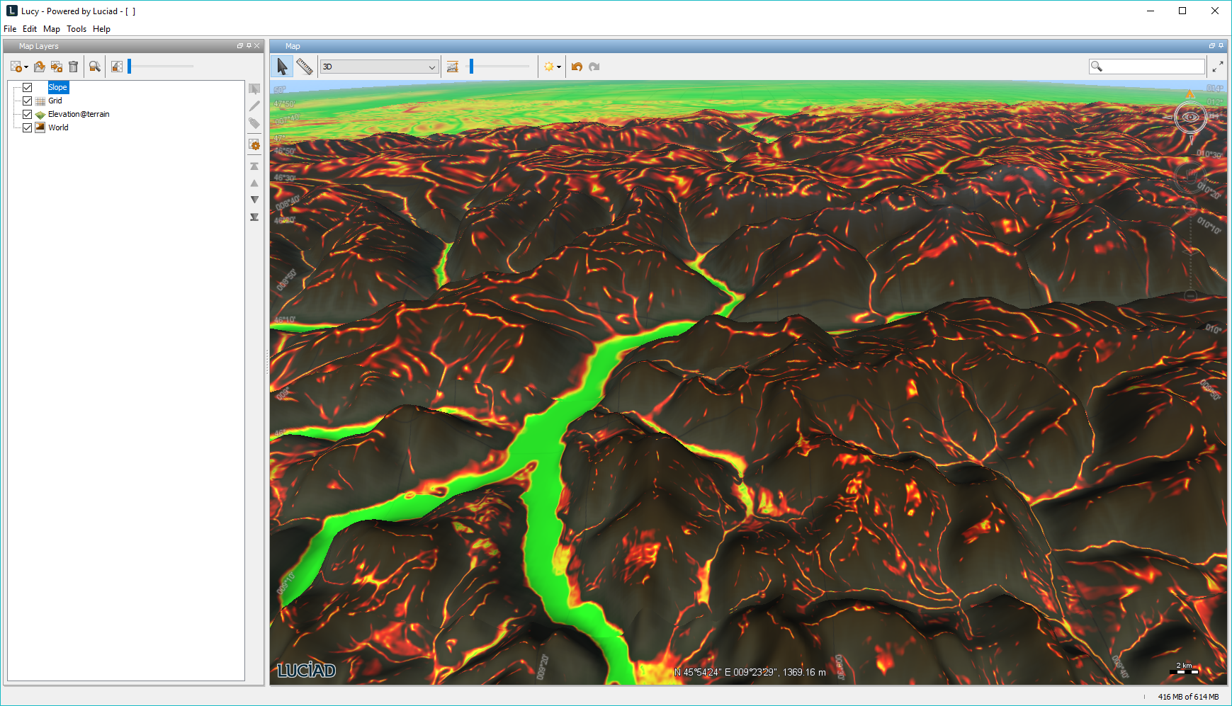
To add a hypsometric raster layer, select Tools→ Hypsometry from the main menu, and select the layer type you want. To switch the layer type, repeat the previous step. The previously created layer is replaced with the new layer.
- Map-centric Lucy
-
To select a hypsometric layer, select Data → New Layer → Hypsometry icon from the main menu.
Adding a shading layer
Select Tools→ Hypsometry → Hill shading from the main menu. A Hill shading layer is added to the map layer overview. The terrain slope is computed, and hill shading is applied to the currently visible map. The terrain shading is based on the direction and angle of inclination of a light source. You can change that direction and inclination on the Hypsometry tab of the Hill shading layer properties panel.

Enter a light reference direction in azimuth degrees or manipulate the arrow in the disk. To change the inclination, enter an alternative inclination in degrees, or manipulate the arrow in the quarter disk on the right.
Lucy applies shading to the map with color variation going from dark for shaded areas to transparent for lit areas. The layer properties panel allows you to choose alternative colors in the Colors bar. For more information about using the color bar, see The color bar.
Adding an azimuth layer
Select Tools→ Hypsometry → Azimuth from the main menu. An Azimuth layer is added to the map layer overview, and the azimuth is visualized for all terrain points on the map. The point coloring is based on the angle between the given reference direction and the orientation of the terrain.
To change the reference direction, open the properties of the Azimuth layer, and go to the Hypsometry tab.
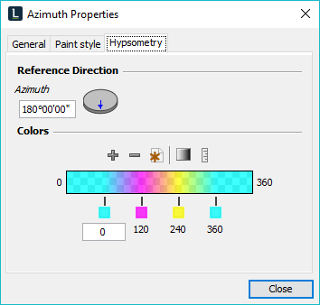
You can enter a reference direction in azimuth degrees or manipulate the arrow in the disk.
Lucy visualizes terrain azimuths on the map as colors from a graduated color scheme. The layer properties panel allows you to choose alternative colors in Colors color bar. For more information about using this bar, see The color bar.
Adding an orientation layer
Select Tools→ Hypsometry → Orientation from the main menu. An Orientation layer is added to the map layer overview, and visualizes the angles of steepest descent of the terrain with reference to a given direction on a Cartesian plane.
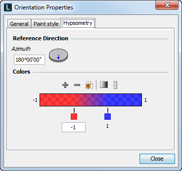
To change the reference direction, open the properties of the Orientation layer, and go to the Hypsometry tab. Enter a reference direction in azimuth degrees or manipulate the arrow in the disk.
Lucy visualizes terrain orientation on the map in the colors of a graduated color scheme. The layer properties panel allows you to choose alternative colors in the Colors bar. For more information about using the color bar, see The color bar.
Adding a slope layer
Select Tools→ Hypsometry → Slope from the main menu. A Slope layer is added to the map layer overview, and visualizes a computed terrain slope degree in a range of colors. The computed values range from 0 for horizontal terrain to larger values for increasingly sloping terrain.
To arrive at this result, the Terrain Analysis Engine computes the angle between the given reference direction and the direction perpendicular to the terrain (the normal).
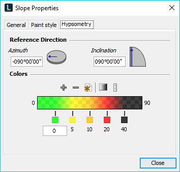
You can change the reference direction and inclination for the slope computation in the layer properties panel. Enter the direction in azimuth degrees or manipulate the arrow in the disk. To change the inclination, enter an alternative inclination in degrees, or manipulate the arrow in the quarter disk on the right.
|
If you change the inclination to an angle other than 90 degrees, so that the reference direction no longer points up, the slope will be visualized inaccurately. |
Lucy visualizes slope on the map in the colors of a graduated color scheme. The layer properties panel allows you to choose alternative colors in the Colors bar. For more information about using the color bar, see The color bar.
Adding a ridges and valleys layer
Select Tools→ Hypsometry → Ridges and valleys from the main menu. A Ridges and valleys layer is added to the map layer overview. It visualizes how strongly the terrain deviates from a locally fitted plane.
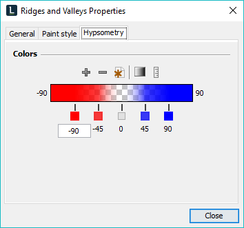
Lucy visualizes ridges and valleys on the map in the colors of a graduated color scheme. High ridges are blue, and deep valleys are red. The layer properties panel allows you to choose alternative colors in the Colors bar. For more information about using the color bar, see The color bar.
Calculating Line-of-sight and object visibility
Lucy and Lucy Map Centric allow you to calculate and display:
-
Line-of-sight coverages
-
Point-to-shape visibility
|
The terrain elevation analysis (TEA) functionality is only applicable to data with terrain elevation information, as provided by DTED and DMED files for example. In the following sections, it is assumed that terrain elevation data is loaded and displayed in the map view. |
Calculating and displaying a line-of-sight coverage
The line-of-sight (LOS) coverage is the area that is visible from a point (for example a radar). For more information, see About LOS coverages.
To calculate the LOS coverage for a point:
-
If it is not already there, add the point to the map. You can add a point object in a drawing layer, for instance, or you could add a point displaying a military symbol.
-
Right-click the icon with the point object, and select Add line-of-sight coverage from the options menu. A Line-of-sight layer is added to the layer tree, and the LOS coverage is displayed on the map.
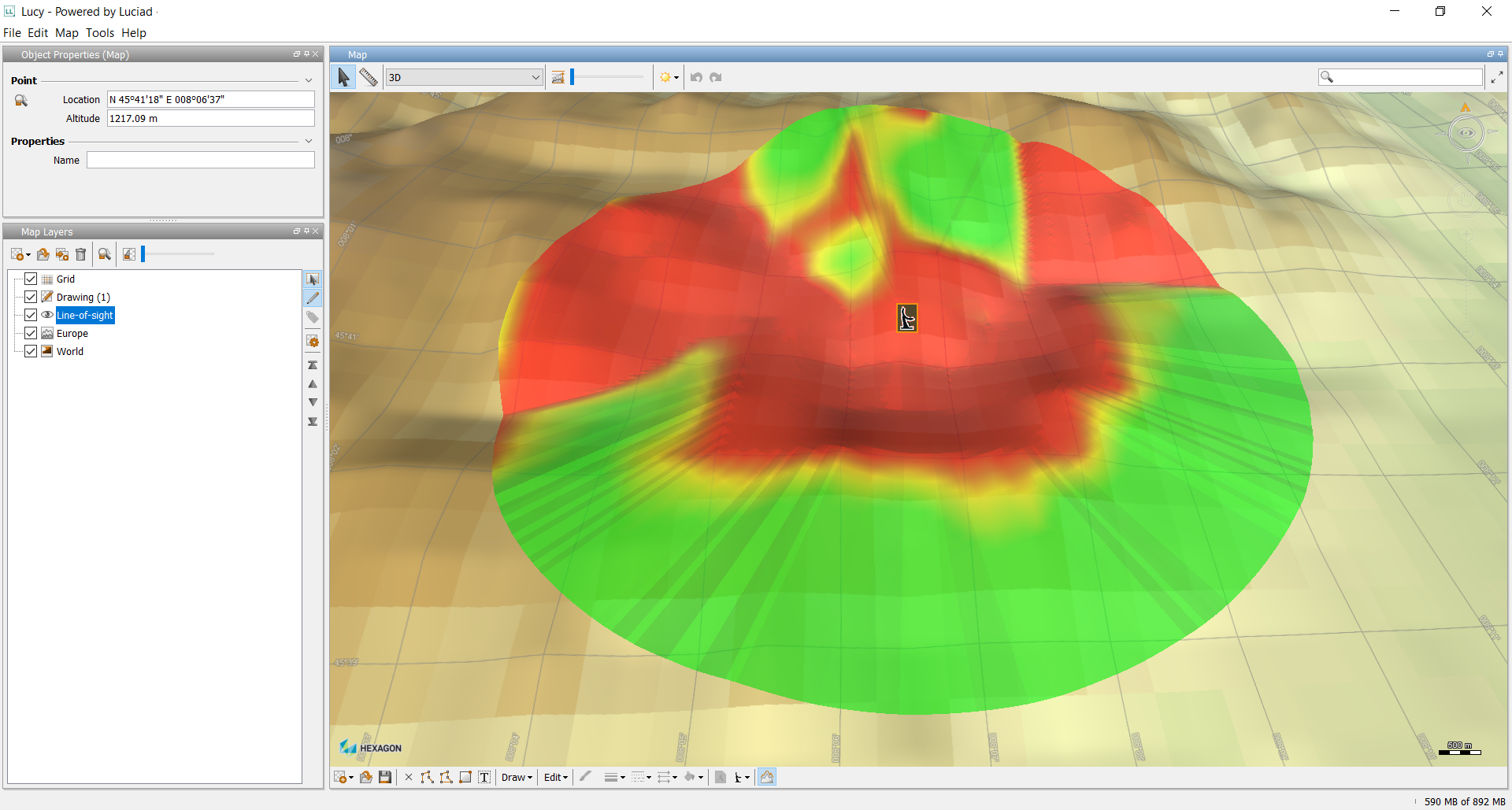
Moving the point of observation
To assess the impact of moving your observation point on object visibility, select the base of the observation point on the map, and drag it to a new map position.
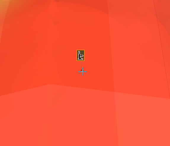
The LOS coverage adapts to the new positions while you are moving the observation point.
Modifying the height-to-color mapping
The colors represent the height at which objects are visible or invisible from the observation point.
Each color is mapped to a specific height range. You can change the applicable heights or map distinct colors to those heights.
To change the color mapping:
-
Right-click the Line-of-sight layer in the Map Layers list, and select Properties.
-
In the Properties dialog box, go to the Line-of-sight tab, and use the color bar to adjust the color settings.
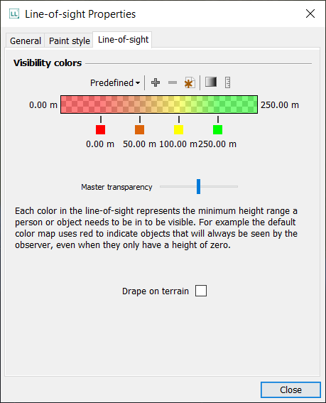
For more information about using the color bar, see The color bar.
By default, the LOS coverage colors are set to display height-based visibility as a color progression over a height range. This is the pre-defined Height based visibility color mapping.
The other pre-defined color range is ground-based. The LOS coverage areas with objects visible at ground level are colored in red, while the rest of the LOS coverage remains transparent. To change the LOS coverage colors to ground-based visibility, select Ground visibility from the Predefined drop-down menu.
To increase or decrease the transparency of colored areas in the LOS coverage, drag the Master transparency slider to the right or left.
Draping the LOS coverage on terrain
To drape the LOS coverage on the loaded terrain:
-
Right-click the Line-of-sight layer in the Map Layers list, and select Properties.
-
In the Properties dialog box,select the Drape on terrain check box.
Changing LOS coverage calculation parameters and updating the LOS coverage
A LOS coverage is the result of a visibility calculation. You can change the way it is calculated by adjusting the calculation parameters.
To change the calculation parameters:
-
On the map, click anywhere in the LOS coverage area surrounding the observation point.
The LOS coverage colors disappear, and the Line-of-sight panel opens.
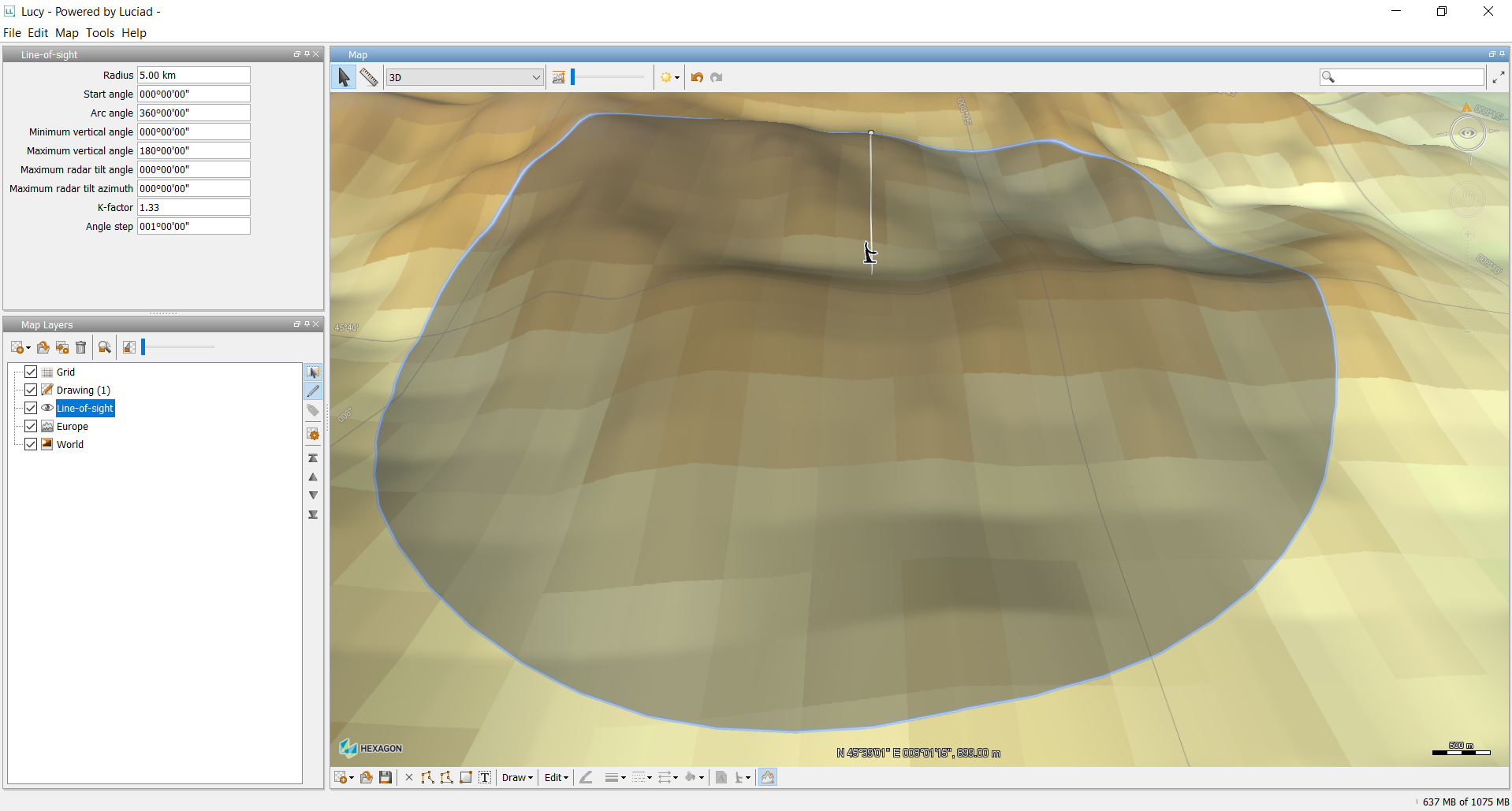
-
Adjust the parameters:
-
Radius: the radial extent of the coverage area.
You can also drag the circumference of the LOS coverage outwards or inwards on the map to adjust the LOS coverage radius
-
Start angle: the starting angle of the arc which defines the horizontal coverage area.
-
Arc angle: the angular extent of the arc which defines the horizontal coverage area.
-
Minimum vertical angle: The angular lower bounds for the cone of silence around the observer.
-
Maximum vertical angle: The angular upper bounds for the cone of silence around the observer.
-
Maximum radar tilt angle: the maximum tilt angle of the observation radar.
-
Maximum radar tilt azimuth: the azimuth where the maximum radar tilt angle occurs
-
K-factor: a factor indicating the reflection of radar waves on the atmosphere.
-
Angle step: the angular discretization step used to find the computation points
-
-
Press Enter after each parameter change, and the displayed LOS coverage will adapt to the new calculation parameters.
Calculating and displaying point-to-shape visibility
Lucy and Lucy Map Centric allow you to visualize and track the visibility of a shape object to an observer. The shapes, or parts of the shape, are marked with a color that indicates their visibility from a specific vantage point on the map.
Start tracking the visibility of a shape
First, you need to set up the observer, by marking a particular point shape on the map.
To add an observer point:
-
If it is not already there, add the point to the map. You can add a point object in a drawing layer, for instance, or you could add a point displaying a military symbol.
-
Right-click the icon with the point object, and select Mark as observer from the options menu.
An observation layer is added to the layer tree, with an Observers and Observation results sub-layer. An eye icon is added to the selected map point.
|
If you are planning to create multiple observer points, give each point a specific display name in the object Name property. It will help you distinguish them when you are assigning observer points to observed shapes. To change the size of the eye icons, you can open the properties of the Observers layer, and change the icon size on the Paint style tab. |
Next, you need to indicate which shape you want to observe.
To mark a shape for observation:
-
If it is not already there, add the shape to the map. You can add a shape object in a drawing layer, for instance. You can mark points, polylines and polygons for observation.
-
Right-click the shape, and select the Observe by <assigned observer name> item from the options menu. If there are multiple observers, there are multiple Observe by options to select from.
-
De-select the shape to see which colors are applied to it. By default, red indicates that a shape part is invisible from the observer point. Green indicates that a shape part is visible from the observer point.
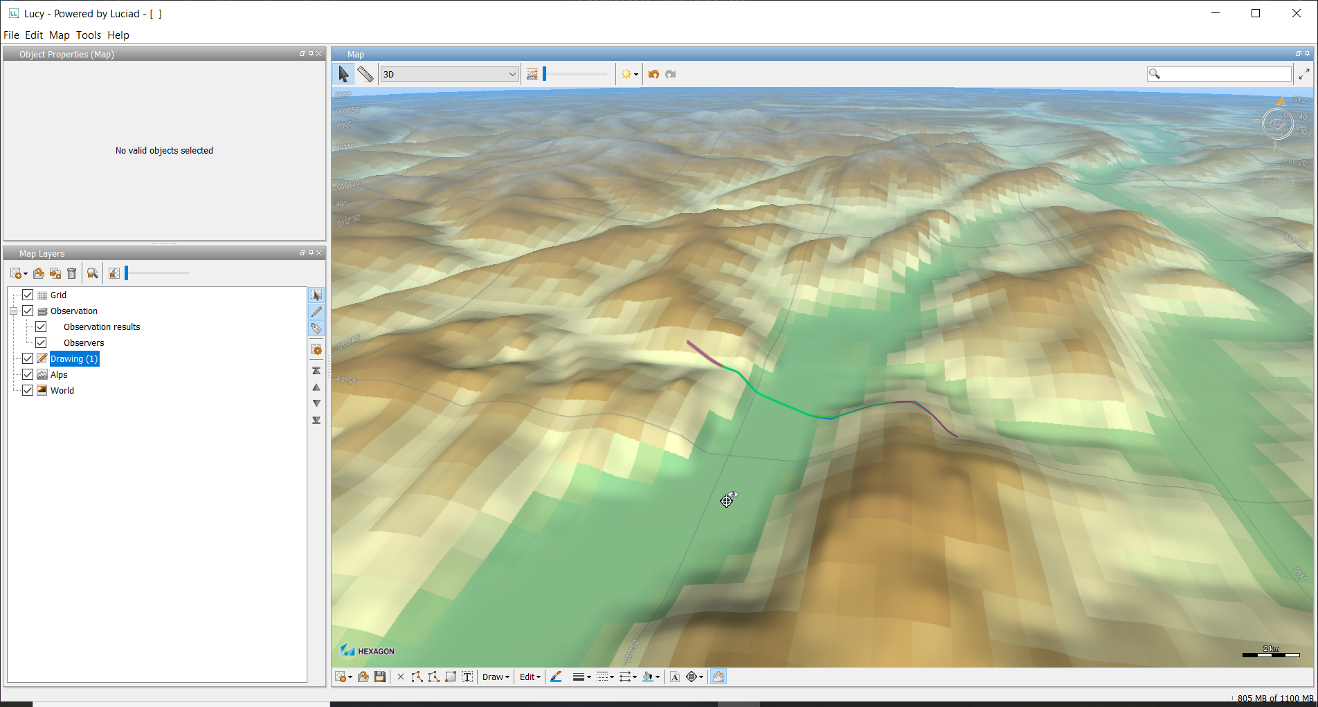
For more information about the visibility colors, see Modifying the visibility-to-color mapping
|
If you are observing a 3D shape, the visibility of the shape is displayed at ground level. If you are observing a shape from multiple observer points, the visibility calculation results are combined into one result. |
When you move the shape or the observer point, by playing back a flight track in the previewer for instance, the colors of the tracked shape adapt to indicate the changing visibility.
Tracking the objects observed by an observer
To find out which objects a particular point is observing, select the eye icon of an observer point. The Object Properties panel shows a list of observed shape objects.
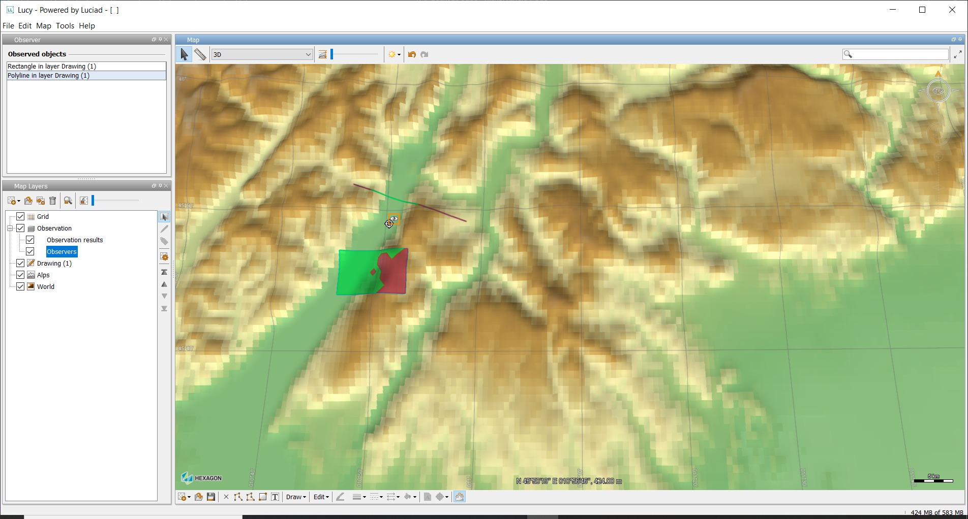
Modifying the visibility-to-color mapping
The colors represent the visibility of the observed shape to the object.
Each measure of visibility is mapped to a default color:
-
Visible: visible shape areas are mapped to green.
-
Invisible: invisible shape areas are mapped to red.
-
Uncertain: if the result of the visibility calculation is uncertain for a shape area, it has a yellow color.
-
Outside shape: areas outside the shape are colored transparently.
You can map distinct colors to those visibility values.
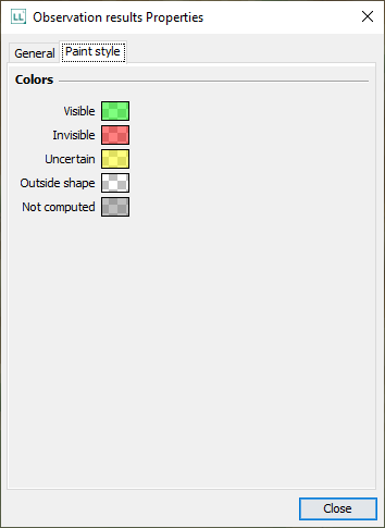
To change the color mapping:
-
Right-click the Observation results sub-layer in the Map Layers list, and select Properties.
-
In the Properties dialog box, go to the Paint style tab, click the colored boxes next to the visibility ratings, and select another color from the Choose a color dialog box.
Stopping observations for visibility
To stop an observer:
-
Right-click the original icon with the observer point.
-
Select Unmark as observer from the options menu.
All observation results for this observer are removed from the map.
To stop the observation of a shape:
-
Right-click the shape.
-
Select the Stop observing by option from the menu.
The observation results for the selected observer are removed from the map.
Alternatively, you can:
-
Select the eye icon of the observer point.
-
Right-click the shape in the Observed objects list of the Object Properties panel
-
Click the Stop observing option
To remove all observations at once, delete the Observations layer.
Using the Terrain Analysis Engine in Lucy GXY
In Lucy GXY, you can calculate and display:
-
Elevation contours
-
Extreme points
-
Shape-to-shape visibility
-
Line-of-sight (or point-to-area) coverage
-
Hypsometric rasters
-
Viewsheds
In addition, it is possible to:
-
View terrain data in the profile view
-
View terrain data in the vertical view
-
Measure distances taking the terrain elevations into account
-
Draw objects following the terrain elevation
When the Terrain Analysis Engine is installed, you can open the following .tea. files using the File→ Open menu:
-
Contours files with extension *.tea.cnt
-
Extreme points files with extension *.tea.ext
-
Line-of-sight files with extension *.tea.los
-
Visibility files with extension *.tea.vis
Each of these files contain the results of the TEA calculations that are described in the following sections.
Calculating and displaying elevation contours in Lucy GXY
To calculate the elevation contours of an area on the map, select the Tools→ Terrain Analysis→ Contours menu item. The Contours panel appears in the top left corner of the application window and a Terrain Contours layer is added to the layer tree with
an empty Contour layer that is used to store the contour calculations. It is possible to add separate contour layers for each
calculation by clicking on the ![]() icon in the bottom left corner of the Contour panel. Make sure to select the appropriate layer in the layer tree when calculating
new elevation contours. The title of the panel shows the selected layer. Figure 98, “The Contours panel” shows the Contours panel.
icon in the bottom left corner of the Contour panel. Make sure to select the appropriate layer in the layer tree when calculating
new elevation contours. The title of the panel shows the selected layer. Figure 98, “The Contours panel” shows the Contours panel.
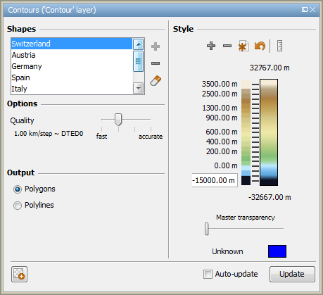
The next sections describe the functionality provided by the Contours panel.
Selecting shapes
The Shapes section contains a list of shapes to which the contour calculation applies. First select one or more shapes in the map view and then click on the icon with the plus sign to add the selected shapes to the list. Note that you can only select shapes that represent an area such as a polygon, sector, or an area of interest. It is also possible to add shapes from the map view to the Shape list by right-clicking on the selected shapes and selecting Terrain Analysis→ Add to contour shape list.
To delete shapes from the list, select the shape in the list and click on the icon with the minus sign. To clear the list click on the icon with the brush. You can also fit the map to a shape or center a shape on the map by selecting the shape in the list, right-clicking, and selecting the corresponding menu item.
Setting the quality level
The Options section contains a slider that allows you to set the quality level for the calculation. The four predefined levels are applicable to the type of data that is loaded. The four levels differ in the distance interval that is used to retrieve the elevation values and are defined as follows:
-
10.0 Km/step, corresponding to the resolution of a DMED raster
-
1.00 Km/step, corresponding to the resolution of a DTED level 0 raster
-
0.10 Km/step, corresponding to the resolution of a DTED level 1 raster
-
0.03 Km/step, corresponding to the resolution of a DTED level 2 raster
Note that with a higher quality level the accuracy of the calculation is better but the calculation time is longer.
Defining the altitude intervals and color settings
The Style section allows you to view and edit the altitude intervals and the color settings as described in The color bar. With the altitude intervals you define for which elevation values contours are calculated. The color settings are used to display areas that have an elevation value within one range of defined elevation values. The grey areas in Figure 99, “A map with DTED data and calculated contours for the Italy country shape”, for example, represent the areas with a height between 1800.00 and 2800.00 m. The Unknown box shows the display color of areas that have no elevation data. Click on the color box to open the color selector and change the color as described in The color selector.
Updating the calculation
When the shapes and style settings are defined you can calculate and display the elevation contours by clicking on the Update button in the bottom right corner of the Contours panel. The calculated contours are added to the active contours layer and displayed in the map view. Select the Auto-update check box to automatically update the elevation contours when the settings are changed. Figure 99, “A map with DTED data and calculated contours for the Italy country shape” shows a map with DTED data and calculated contours for the defined Area of Interest.
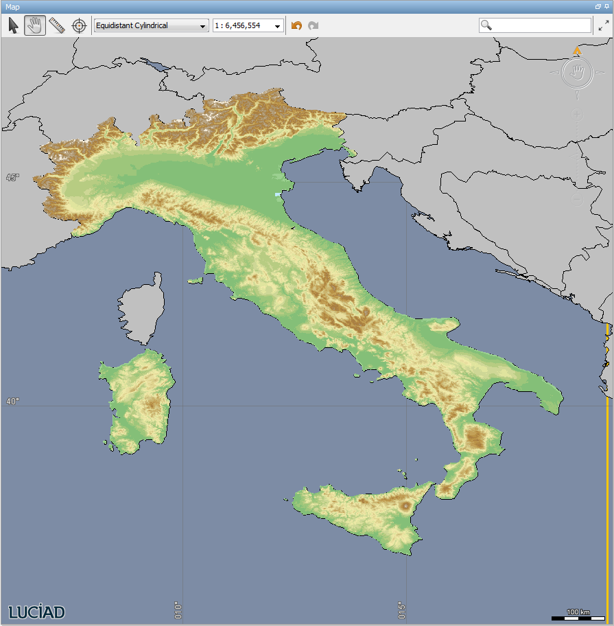
Calculating and displaying extreme points
The extreme points are the lowest and the highest points in an area. To calculate the extreme points of an area, select the
Tools→ Terrain Analysis→ Extreme Points menu item. The Extreme Points panel appears in the top left corner of the application window and an Extreme points layer is added to the layer tree. The
Extreme points layer first contains an empty layer that is used to store the extreme points calculation. It is possible to
add separate Extreme points layers for each calculation by clicking on the ![]() icon in the bottom left corner of the Extreme Points panel. Make sure to select the appropriate layer in the layer tree when
calculating new extreme points. The title of the panel shows the selected layer. Figure 100, “The Extreme Points panel” shows the Extreme Points panel.
icon in the bottom left corner of the Extreme Points panel. Make sure to select the appropriate layer in the layer tree when
calculating new extreme points. The title of the panel shows the selected layer. Figure 100, “The Extreme Points panel” shows the Extreme Points panel.
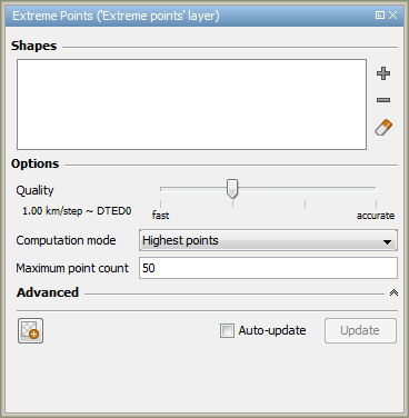
The next sections describe the functionality provided by the Extreme Points panel.
Selecting shapes
The Shapes section contains a list of the shapes to which the extreme points calculation applies. First select one or more shapes in the map view and then click on the icon with the plus sign to add the selected shapes to the list. It is possible to select any object, for example points, lines, sectors, or an area of interest. It is also possible to add shapes from the map view to the Shape list by right-clicking on the selected shapes and selecting Terrain Analysis→ Add to extreme point shape list.
To delete shapes from the list, select the shape in the list and click on the icon with the minus sign. To clear the list click on the icon with the eraser. You can also fit the map to a shape or center a shape on the map by selecting the shape in the list, right-clicking, and selecting the corresponding menu item.
Setting the calculation options
The Options section contains a slider that allows you to set the quality level for the calculation as described in Setting the quality level.
With the Computation mode drop-down list you can determine whether to calculate the lowest or the highest points. In the Maximum point count text box you can enter the maximum number of points to calculate.
In the Advanced section you can define the separation height and distance between two points to ensure that the calculated points differ distinctly and to avoid the calculation of too many or too few points in an area. Figure 101, “Interpretation of the separation height and distance” provides an example on how to interpret the separation height and distance values.
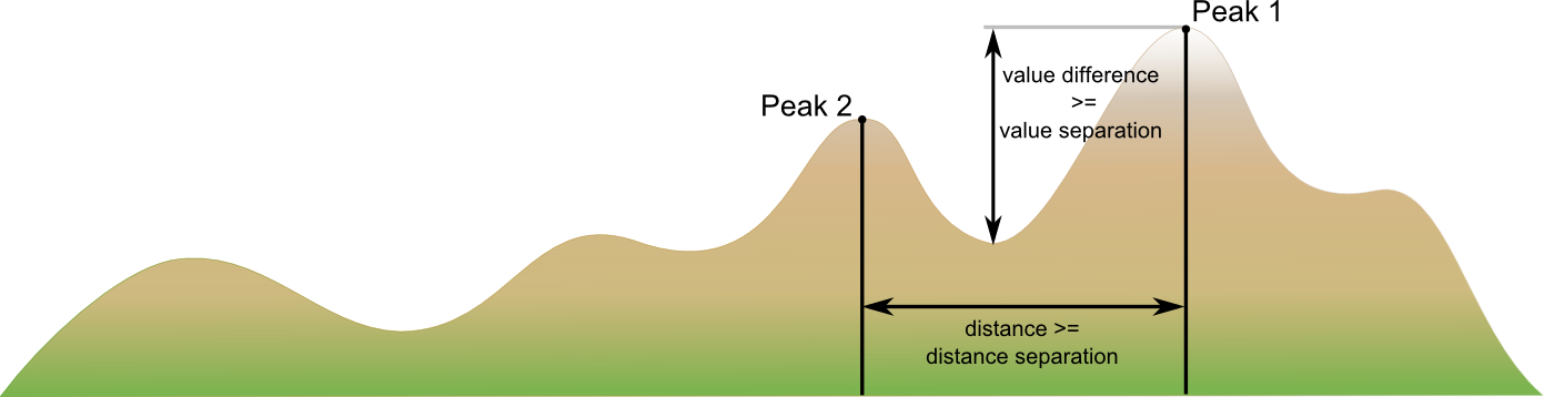
Peak 1 is the highest point in the area. If the height difference between Peak 1 and Peak 2 is equal to or larger than the separation height, Peak 2 is the second highest point in the area. If the height difference is smaller than the separation height, Peak 2 is only considered the second highest point if the distance between Peak 1 and Peak 2 is equal to or larger than the separation distance.
Updating the calculation
When the shapes and other settings are defined you can calculate and display the extreme points by clicking on the Update button in the bottom right corner of the Extreme Points panel. The calculated points are added to the active extreme points layer and displayed in the map view. Select the Auto-update check box to automatically update the extreme points when the settings are changed. Figure 102, “A map with DTED data and calculated extreme points” shows a map with DTED data and calculated extreme points for the defined area. The yellow triangles represent the highest points in the selected area. The labels show the height of each point.
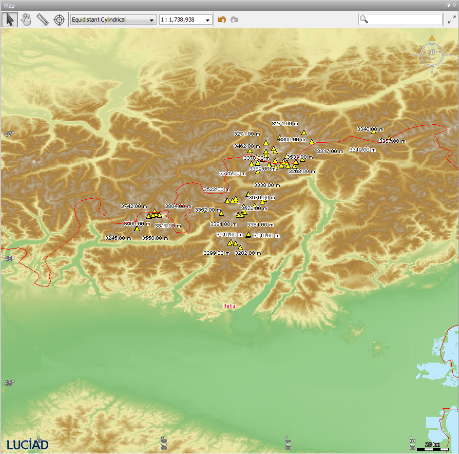
Calculating and displaying the visibility of objects in Lucy GXY
To calculate the visibility from one object to another, select the Tools→ Terrain Analysis→ Visibility menu item. The Visibility panel appears in the top left corner of the application window and a Visibility layer is added to the layer tree. The Visibility
layer first contains an empty layer that is used to store the visibility calculations. It is possible to add separate Visibility
layers for each calculation by clicking on the ![]() icon in the bottom left corner of the Visibility panel. Make sure to select the appropriate layer in the layer tree when
calculating a new visibility. The title of the panel shows the selected layer. Figure 103, “The Visibility panel” shows the Visibility panel.
icon in the bottom left corner of the Visibility panel. Make sure to select the appropriate layer in the layer tree when
calculating a new visibility. The title of the panel shows the selected layer. Figure 103, “The Visibility panel” shows the Visibility panel.
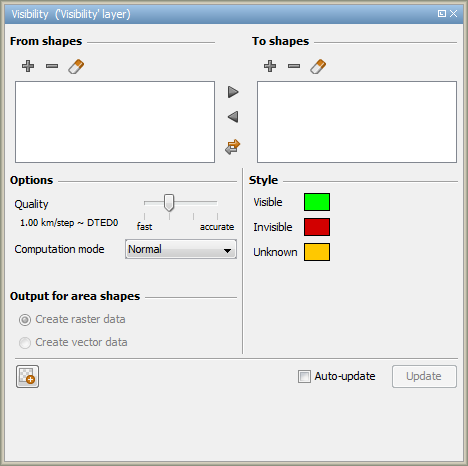
The next sections describe the functionality provided by the Visibility panel.
Selecting objects
The From shapes section contains a list with objects that are the source for the visibility calculation. The To shapes section contains a list with objects that are the target for the visibility calculation. First select one or more objects in the map view and then click on the icon with the plus sign above one the lists to add the selected objects to that list. To delete objects from the list, select the object in the list and click on the icon with the minus sign. To clear the list click on the icon with the brush. It is also possible to add objects from the map view to one of the lists by right-clicking on the selected objects and selecting either Terrain Analysis→ Add to visibility FROM shape list or Terrain Analysis→ Add to visibility TO shape list.
Setting the calculation options
The Options section contains a slider that allows you to set the quality level for the calculation as described in Setting the quality level.
The Computation mode drop-down list allows you to select one of the following computation modes:
-
Normal: computes the visibility between two objects taking the terrain into account as illustrated in Figure 104, “Visibility with the Normal computation mode”. The helicopter is visible from the tower because there is no terrain between the helicopter and the tower.
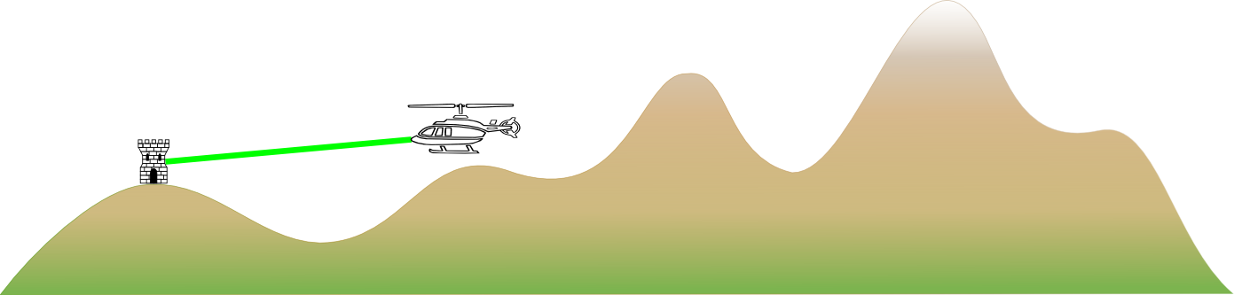 Figure 104. Visibility with the Normal computation mode
 -
Sky in background: computes the visibility between two objects with the sky as background. This mode requires a distance after the target shape in which the terrain is taken into account as possible background. Configure this distance in the Sky distance text box. In this mode, an object can only see another object if there is no terrain between the objects and if there is no terrain behind the target shape for the defined sky distance as illustrated in Figure 105, “Visibility with the Sky in background computation mode”. The helicopter is not visible from the tower because there is terrain behind the helicopter within the defined sky distance.
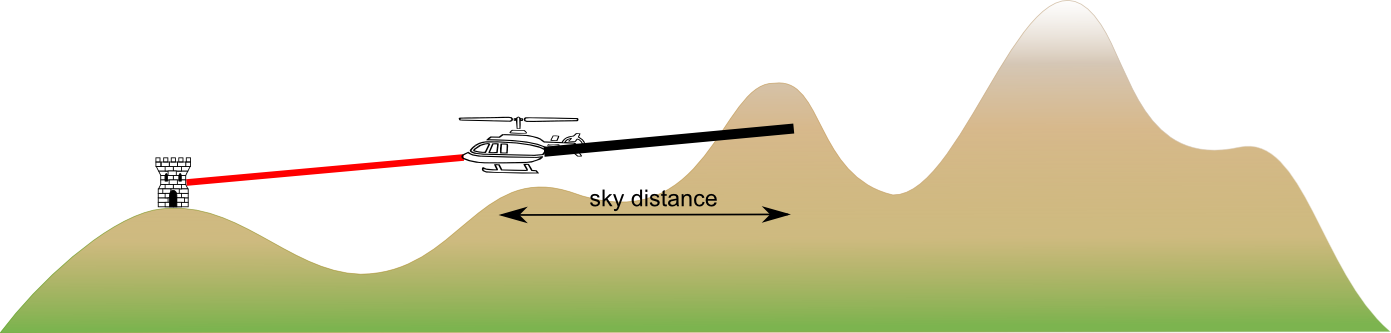 Figure 105. Visibility with the Sky in background computation mode
The calculated visibility can either be raster or vector data as indicated by the check boxes in the Output section. The raster output is slightly more accurate since each pixel is computed for the exact elevation value available in the loaded data. When creating the visibility contour lines for vector output, an extra rounding step is performed which makes the visualization better for small map scales. The computation time is more or less the same for both output modes.
|
Note that the raster output is only used for objects representing an area such as a polygon or sector. |
Defining the color settings
The Style section provides color settings to display the areas on the map where the target object is visible or invisible and for which the visibility is unknown. Click on a color to open the color selector and change the defined color as described in The color selector.
Updating the calculation
When the objects and other settings are defined you can calculate and display the visibility by clicking on the Update button in the bottom right corner of the Visibility panel. The calculated visibility is added to the active visibility layer and displayed in the map view. Select the Auto-update check box to automatically update the visibility when the settings are changed. Figure 106, “The visibility of a polyline from three points on the map” shows a map with the visibility of a polyline from three points on the map. The green line indicates the area where the polyline is visible and the red line the area where the line is invisible. Note that when multiple source objects are selected, the target object is displayed as visible if at least one of the objects can see it.
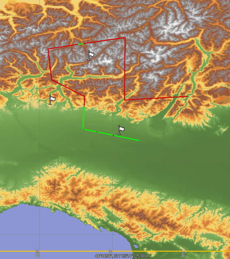
Calculating and displaying a line-of-sight coverage in Lucy GXY
The line-of-sight (LOS) coverage is the area that is visible from a point (for example a radar). To calculate the LOS coverage
of a point, select the Tools→ Terrain Analysis→ Line-of-sight Coverage menu item. The Line-of-sight Coverage panel appears in the top left corner of the application window and a LOS Coverages layer is added to the layer tree. The
LOS Coverages layer first contains an empty layer that is used to store the calculated LOS coverage. It is possible to add
separate LOS Coverage layers for each calculation by clicking on the ![]() icon in the bottom left corner of the Line-of-sight Coverage panel. Make sure to select the appropriate layer in the layer
tree when calculating a new LOS coverage. The title of the panel shows the selected layer. Figure 107, “The Line-of-sight Coverage panel” shows the Line-of-sight Coverage panel.
icon in the bottom left corner of the Line-of-sight Coverage panel. Make sure to select the appropriate layer in the layer
tree when calculating a new LOS coverage. The title of the panel shows the selected layer. Figure 107, “The Line-of-sight Coverage panel” shows the Line-of-sight Coverage panel.
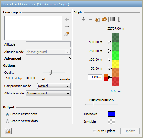
The next sections describe the functionality provided by the Line-of-sight Coverage panel.
Selecting points
The Coverages section contains a list of points to which the LOS coverage calculation applies. First select one or more points on the map and then click on the icon with the plus sign to add the selected points to the list. It is also possible to add points from the map view to the Coverages list by right-clicking on the selected points and selecting Terrain Analysis→ Add to line-of-sight coverage list.
To delete points from the list, select the point in the list and click on the icon with the minus sign. To clear the list click on the icon with the eraser. You can also fit the map to a coverage or center a point on the map by selecting the point in the list, right-clicking, and selecting the corresponding menu item.
By default the 2D position of the selected point is considered with a default altitude of 2 m above ground. To change the altitude, enter the altitude in the Altitude text box and select one of the options from the Altitude mode drop-down list to indicate the reference for the altitude:
-
Above ground: takes the terrain as reference.
-
Above mean sea level: takes the mean sea level as reference.
-
Above object: takes an object as reference. Note that this option is only useful when the reference object does not have a constant altitude, for example a 3D line.
The Advanced section allows you to view and edit the following properties for the coverage area:
-
Location: the 2D location of the point that is the center of the coverage area. Note that you can only edit the location if the layer to which the selected point belongs, is editable.
-
Start angle: the starting angle of the arc which defines the horizontal coverage area.
-
Arc angle: the angular extent of the arc which defines the horizontal coverage area.
-
Max radius: the radial extent of the horizontal coverage area.
-
Min vertical angle: the minimum angle of the vertical coverage area.
-
Max vertical angle: the maximum angle of the vertical coverage area.
Figure 108, “The horizontal properties of a line-of-sight coverage” shows an interpretation of horizontal coverage area properties. For points without an orientation, the start and arc angle are relative to the north. For points with an orientation, for example a flight track, the angle is relative to the orientation.
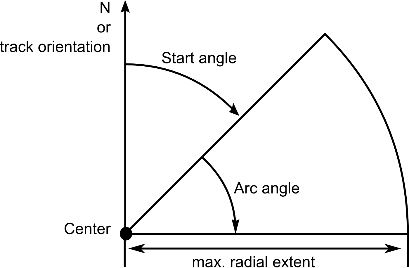
The vertical angles start from 0 at the ground to 180 at zenith as illustrated by Figure 109, “The vertical properties of a line-of-sight coverage”.
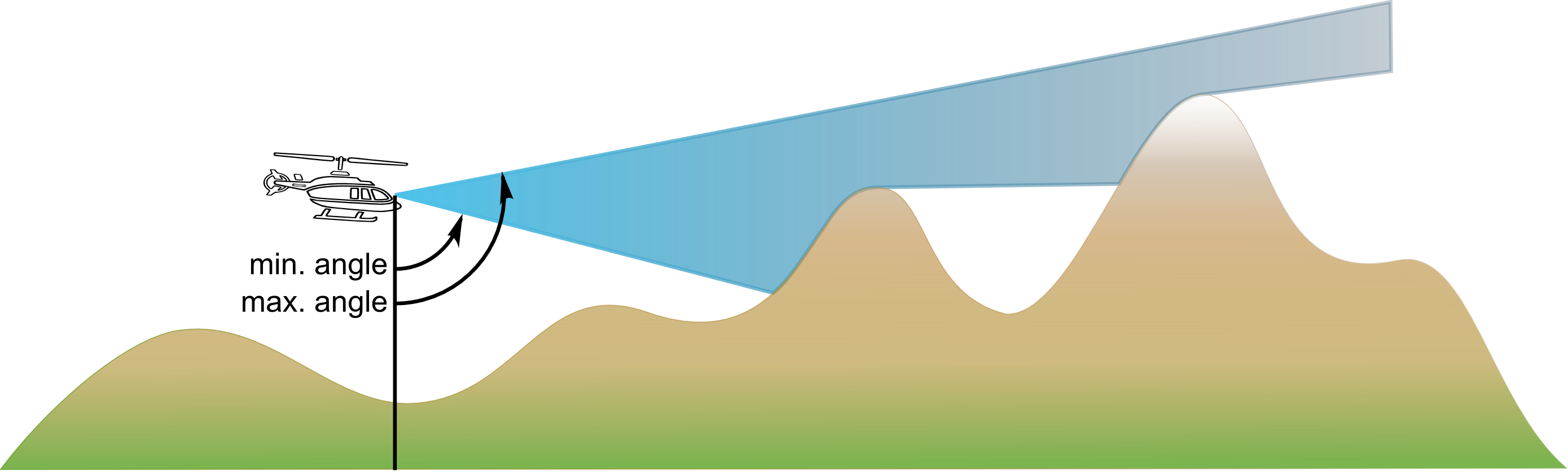
Setting the calculation options
The Options section contains a slider that allows you to set the quality level for the calculation as described in Setting the quality level.
The Computation mode drop-down list allows you to select one of the following computation modes:
-
Normal: computes the minimal height at which an object is visible from the selected point as shown by the green line in Figure 110, “LOS coverage using the Normal computation mode”. The two dotted lines represent the visible area for the pilot in the helicopter.
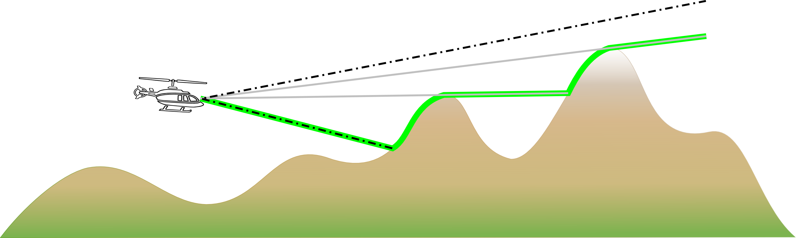 Figure 110. LOS coverage using the Normal computation mode
The Altitude mode drop-down list allows you to select if the result is defined above ground or above mean sea level. Figure 111, “The two different altitude modes” illustrates the different altitude modes.
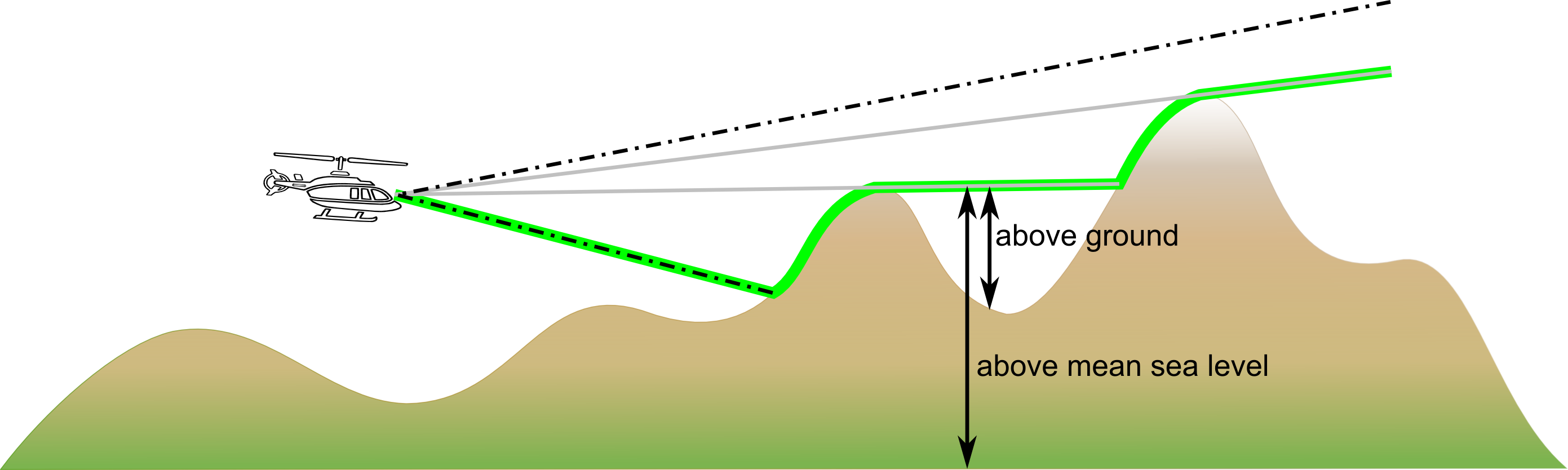 Figure 111. The two different altitude modes
 -
Sky in background: computes the minimal height at which an object is visible from the selected point with the sky as background. The green line in Figure 112, “LOS coverage using the Sky in background computation mode” represents the resulting height. Objects below the green line are not visible or less visible because they are seen with terrain in the background.
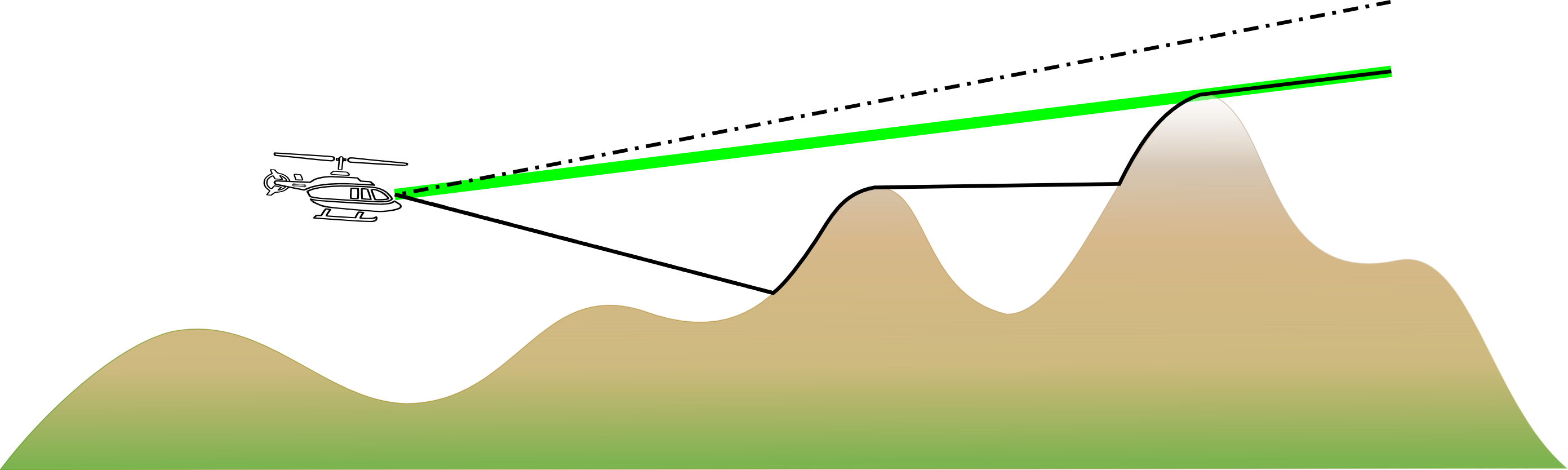 Figure 112. LOS coverage using the Sky in background computation mode
The Altitude mode drop-down list allows you to select if the result is defined above ground or above mean sea level. Figure 111, “The two different altitude modes” illustrates the different altitude modes.
-
Fixed height: computes the visibility of objects at a fixed height and returns three values as shown in Figure 113, “LOS coverage using a fixed height above mean sea level”. The green line corresponds to the points where objects are visible. The red line corresponds to points where objects are invisible due to the obstruction of terrain, while the blue line corresponds to points where objects are invisible due to the cone of silence around the given point. The cone of silence is a cone-shaped region, directly above and below a point, in which nothing is visible.
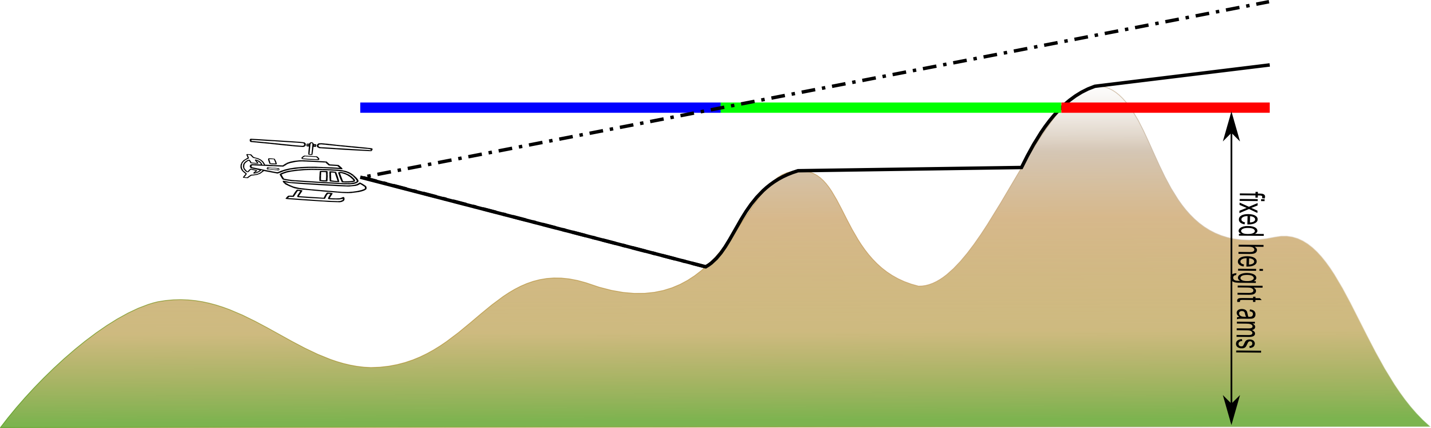 Figure 113. LOS coverage using a fixed height above mean sea level
When selecting the Fixed height mode, enter the value for the height in the Fixed height text box and select with the Fixed height mode drop-down list if the height is above ground or above mean sea level (indicated as amsl in Figure 113, “LOS coverage using a fixed height above mean sea level”). Figure 114, “LOS coverage using a fixed height above ground” shows the visibility of objects at a fixed height above ground.
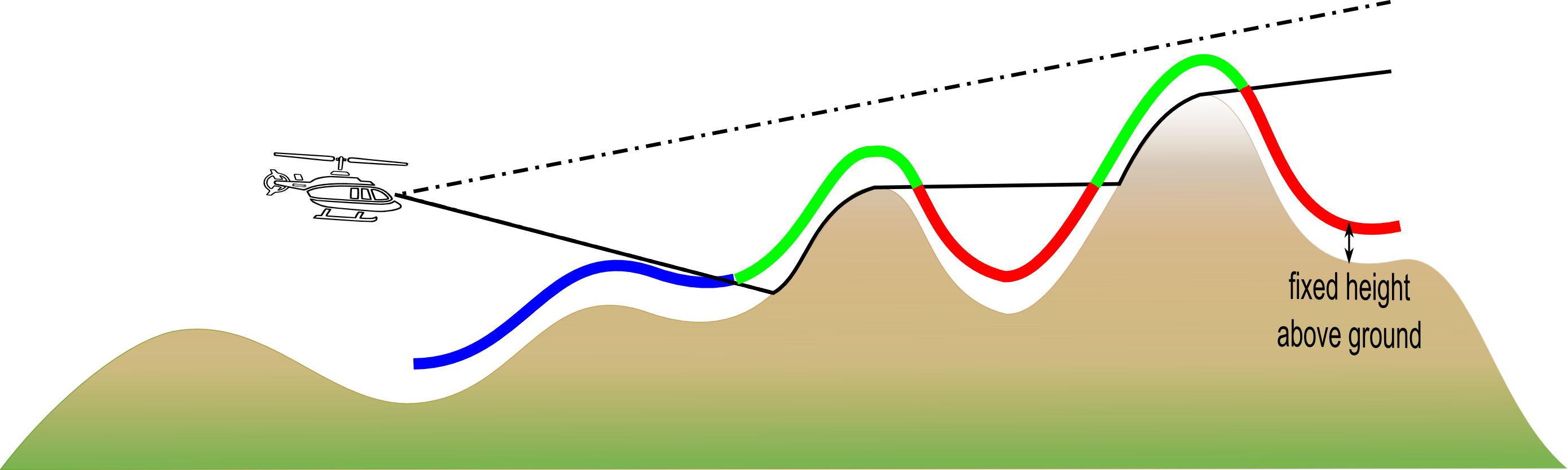 Figure 114. LOS coverage using a fixed height above ground
The resulting LOS coverage can either be raster or vector data as indicated by the radio boxes in the Output section. The raster output is slightly more accurate since each pixel is computed for the exact elevation value available in the loaded data. When creating the visibility contour lines for vector output, an extra rounding step is performed which makes the visualization better for small map scales. The computation time is more or less the same for both output modes.
Defining the altitude intervals and color settings
The Style section allows you to view and edit the altitude intervals and color settings as described in The color bar. When Create raster data is selected in the Output section, an icon with a gradient indication ![]() is added above the color bar. Click on the icon to use gradient colors instead of distinct colors to represent the defined
heights.
is added above the color bar. Click on the icon to use gradient colors instead of distinct colors to represent the defined
heights.
The Unknown box shows the display color of areas that have no elevation data. The Invisible box shows the display color of the area that is invisible. With the altitude intervals you define for which elevation values contours are calculated. The color settings are used to display areas that have an elevation value within one range of defined elevation values. The yellow areas in Figure 115, “The line-of-sight coverage for a point on the map”, for example, represent the areas with a height between 50.00 m and 100.00 m. Click on the color box to open the color selector and change the colors as described in The color selector.
Updating the calculation
When the points and other settings are defined you can calculate and display the LOS coverage by clicking on the Update button in the bottom right corner of the Line-of-sight Coverage panel. The calculated LOS coverage is added to the active LOS coverage layer and displayed in the map view. Select the Auto-update check box to automatically update the LOS coverage when the settings are changed. Figure 115, “The line-of-sight coverage for a point on the map” shows a map with the LOS coverage for a point on the map with a radius of 20 km. The red, orange, and yellow areas are all lower than 100 m, the green areas are higher than 100 m. There is no invisible area.
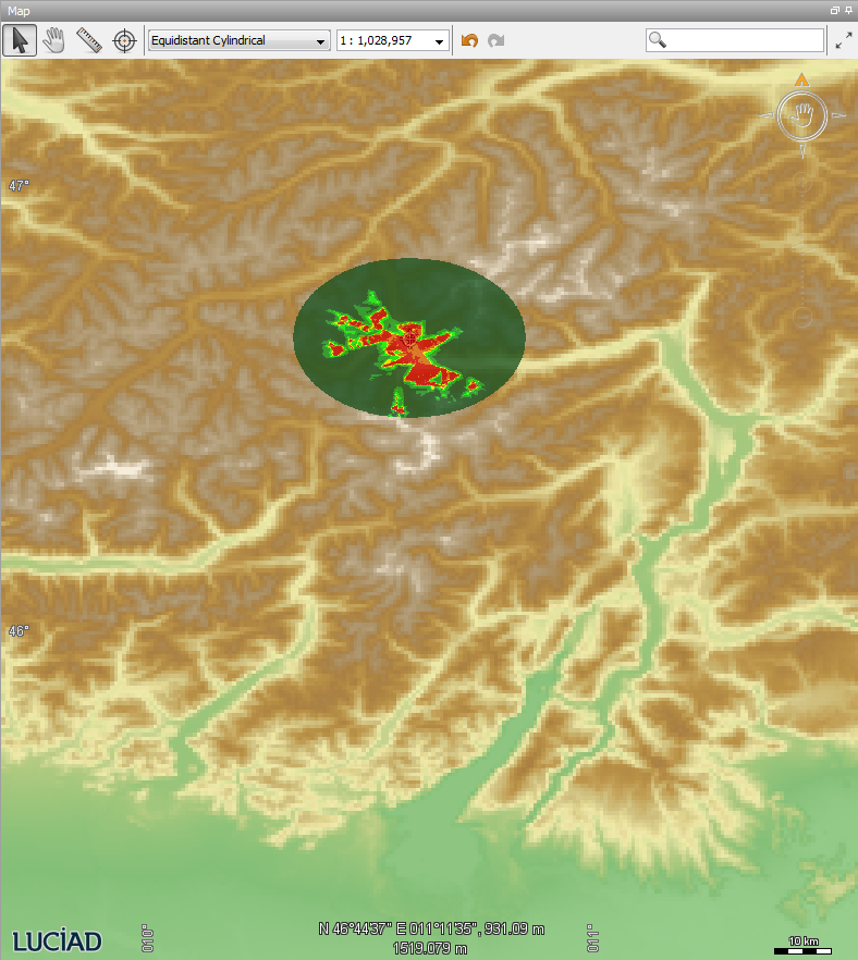
Calculating and displaying hypsometric rasters in Lucy GXY
To calculate hypsometric rasters from elevation data, select the Tools→ Terrain Analysis→ Hypsometry menu item. The Hypsometry panel appears in the top left corner of the application window.
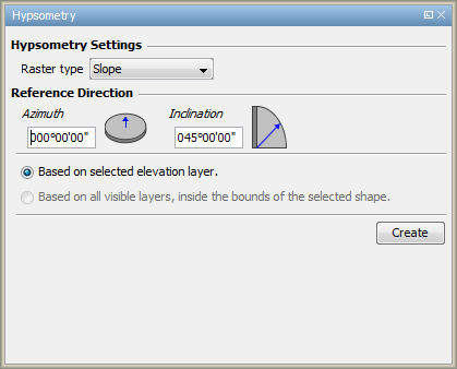
The next sections describe the functionality provided by the Hypsometry panel.
Defining a hypsometric raster
The Hypsometry Settings section contains a Raster type drop-down box from which you can select one of the following raster types:
-
Slope: computes the cosine of the angle between the given reference direction and the normal. The color settings result in a shaded terrain in the map view with the sun positioned in the reference direction.
-
Slope Angle: computes the angle between the given reference direction and the line perpendicular to the terrain (the normal). The color settings represent the slope of the terrain in the map view.
-
Orientation: computes the cosine of the Orientation Angle (see below).
-
Orientation Angle: computes the angle between the given reference direction and the orientation of the terrain.
-
Ridges: computes the ridges of the terrain.
-
Valleys: computes the valleys of the terrain.
-
Ridges and Valleys: computes the ridges and valleys of the terrain.
|
The computation of slope and orientation is faster than the computation of the slope angle and orientation angle but the result is less accurate. |
For the slope and slope angle, define the reference direction by entering a value for the Azimuth and the Inclination. For the orientation and orientation angle, define the reference direction by entering a value for the Azimuth.
Creating a hypsometric raster
After defining the raster settings, select one of the radio buttons in the bottom of the panel to:
-
Base the raster on the selected elevation layer. Note that you first have to select a layer containing elevation data in the layer tree. The hypsometric raster is created directly from the elevation raster of the selected layer.
-
Base the raster on all visible layers inside the bounds of the selected shape. Note that you first have to select a shape in the map view. An elevation raster is first created based on the visible layers in the bounds of the selected shape and then the hypsometric raster is created from the created elevation raster.
Click on the Create button in the bottom right corner of the panel to create a layer with GeoTIFF data for the new hypsometric raster. The raster layer is added to the layer tree and the raster is displayed in the map view. Figure 117, “A hypsometric slope in the map view” shows a hypsometric slope with an azimuth of 30 degrees and an inclination of 15 degrees.
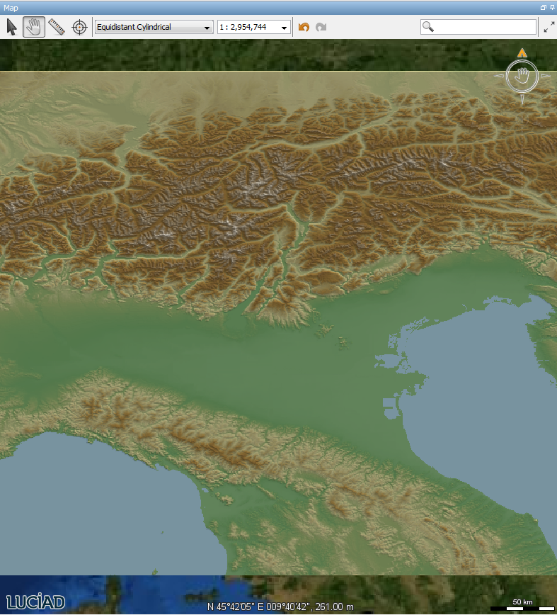
Updating a hypsometric raster
To view and edit the properties of a hypsometric raster, select the corresponding layer in the layer tree and open the Object properties panel of the layer as described in The layer properties panel. The Paint style tab allows you to change the Paint Style Properties as described in The layer paint style. The Reference Direction allows you to change the defined raster settings as described in Defining a hypsometric raster. Open the Colors tab to change the current color settings as described in The color bar. Figure 118, “The Object properties panel of a hypsometric slope” shows the Object properties panel of the hypsometric slope that is shown in Figure 117, “A hypsometric slope in the map view”.
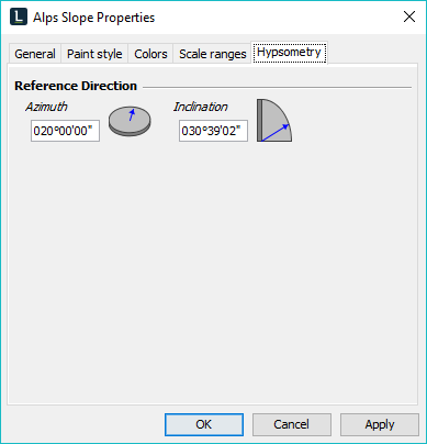
Calculating and displaying the viewshed of 3D scenes
To calculate the viewshed for a given 3D scene, select the Tools→ Terrain Analysis→ Viewshed menu item. The Viewshed panel appears in the top left corner of the application window.
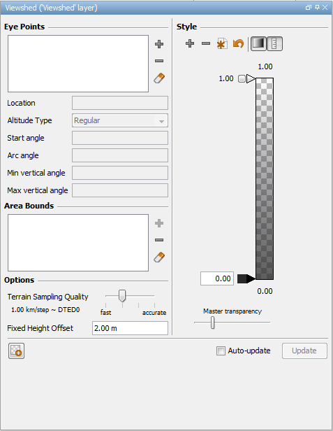
The next sections describe the functionality provided by the Viewshed panel.
Selecting points
The Viewshed section contains a list of points which will act as input for the viewshed calculations. First select one or more points on the map and then click on the icon with the plus sign to add the selected points to the list.
To delete points from the list, select the point in the list and click on the icon with the minus sign. To clear the list click on the icon with the brush. You can also fit the map to a coverage or center a point on the map by selecting the point in the list, right-clicking, and selecting the corresponding menu item.
Right below the list of eye points there is a checkbox to set the altitude type. There are two altitude types:
-
Regular: The reference of the point is used to interpret its height. To edit the height of the point, use the Object Properties panel. This panel can be attained by right clicking the point on the map and selecting Properties.
-
Sun Position: The location of the point is interpreted as the location of the sun. The point will be at infinite height.
The Location text field allows you to change the 2D location of the point. Note that you can only edit the location if the layer to which the selected point belongs, is editable.
The rest of the panel allows you to change section allows you to define a cone of silence around the currently selected eye point.
-
Start angle: the horizontal starting angle of the arc which defines cone of silence.
-
Arc angle: the horizontal angular extent of the arc which defines cone of silence.
-
Min vertical angle: the minimum vertical angle of the cone of silence.
-
Max vertical angle: the maximum vertical angle of the cone of silence.
Note that these values are only used when the Altitude Type of the selected point is set to Regular.
Figure 120, “The horizontal properties of a cone of silence” shows an interpretation of horizontal cone of silence properties.
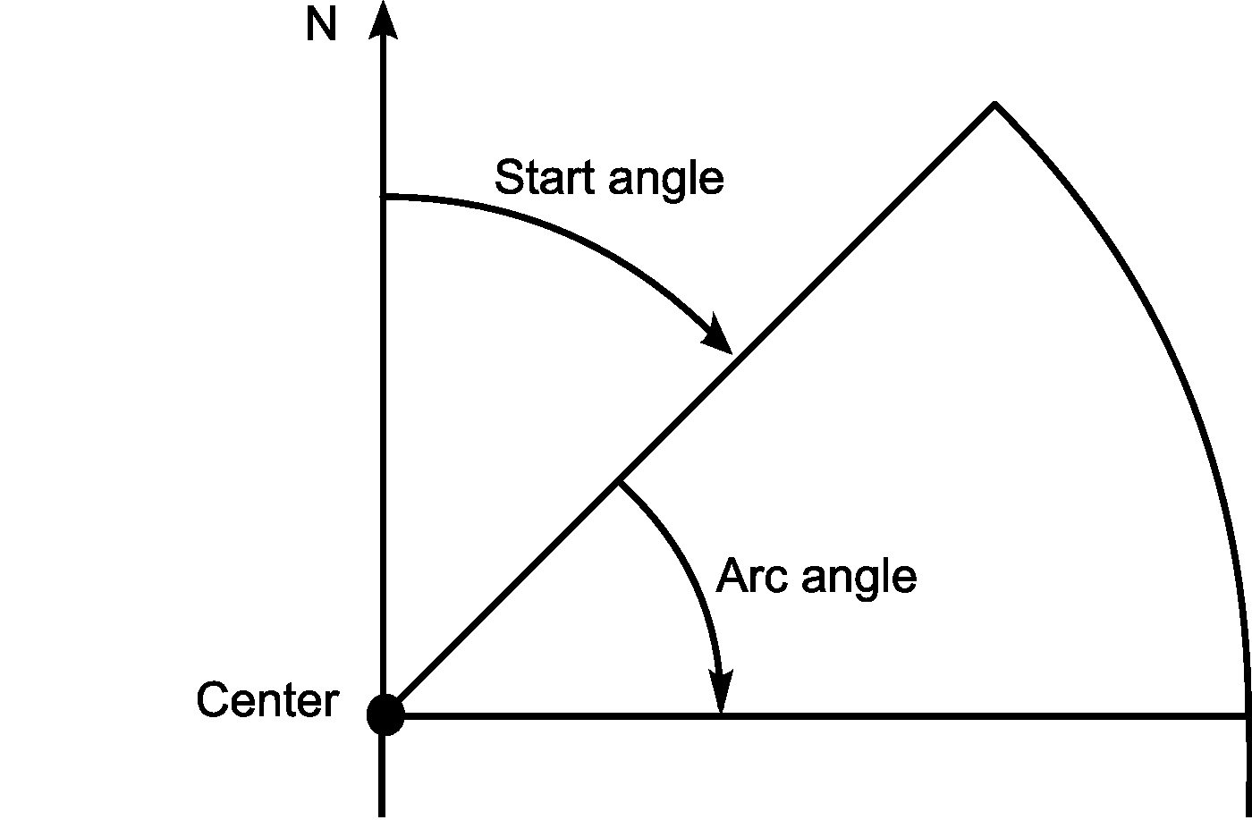
The vertical angles start from 0 at the ground to 180 at zenith as illustrated by Figure 121, “The vertical properties of a cone of silence”.
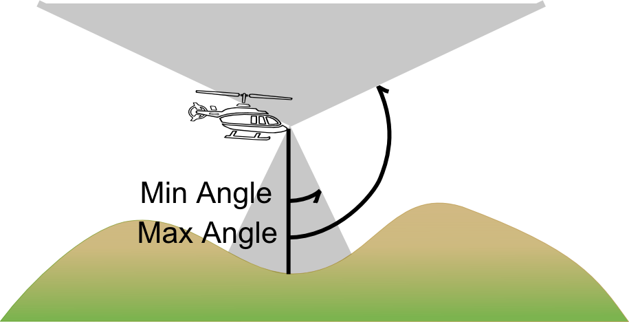
The Area Bounds box is a list of areas in which the viewshed should be visualized. Like for the eye point list, select one or more shapes on the map and then click on the icon with the plus sign to add the selected shapes to the list. To delete shapes from the list, select the shape in the list and click on the icon with the minus sign. To clear the list click on the icon with the brush.
The Terrain Sampling Quality slider can be adjusted to increase or decrease the sampling rate for terrain. This slider only affects the sampling quality of terrain, not buildings and other 3D objects.
The Fixed Height Offset text field can be edited to give a fixed height offset while sampling the viewshed. This fixed height offset will be added to the height of the terrain. Viewshed visibility calculations will happen on this fixed height point for each individual sampling point within the given Area Bounds.
Defining the color settings
The Style section allows you to view and edit the visibility intervals and color settings as described in The color bar. The values on the color bar should be interpreted as levels of visibility. The highest value is 1.0, which represents a fully visible point. 0.0 is the lowest value, which represents a point that is not visible. Anything in between these values can be interpreted as a visibility that is only seen by a few observers. Figure 122, “An example of a color scheme with multiple observers” shows an example of a viewshed that has areas only visible to some observers. In this image, red is fully invisible, orange is visible to one observer and green is visible to both observers.
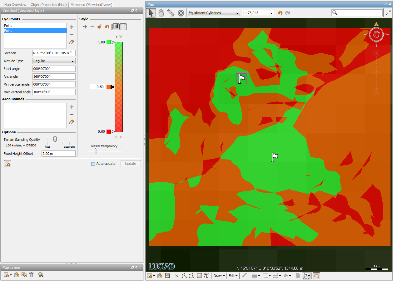
Updating the calculation
When the points and other settings are defined you can calculate and display the viewshed by clicking on the Update button in the bottom right corner of the Viewshed panel. The calculated viewshed raster is added to the active viewshed and displayed in the map view.
Viewshed rasters are multi-leveled and lazy. This means that as you zoom in, the image will become sharper asynchronously.
Select the Auto-update check box to automatically update the viewshed when the settings are changed.
Other TEA functionality
This section describes the functionality that is added by the Terrain Analysis Engine in addition to the functionality described in the above sections.
Viewing terrain data in the profile view
When you are using a 2D map, you can view a terrain in the profile view. To do this, select the Map→ Controls→ Profile view menu item. A Profile panel appears under the map view. Point the mouse to a location on the map to display the altitude of that location in a box next to the mouse pointer. Click on the map and drag the mouse over the map to see the profile of the selected terrain in the Profile panel. Figure 123, “The Profile view” shows the Profile view. The altitudes of the start and end point of the terrain are shown left and right of the profile.
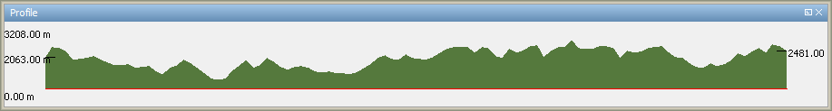
Click in the Profile view to add a slider that controls the terrain location in both the map and profile view and shows the corresponding altitude.
When you are using a 3D map, you can access the profile view functionality in the vertical view. For more information about the vertical view, see Displaying shape height in a vertical view. During the creation of a polyline, the underlying profile is automatically updated.
Measuring distances over terrain
When the Terrain Analysis Engine is installed, the default functionality to measure distances on the map is enhanced by adding the possibility to take the terrain elevation data into account. The Ruler panel as described in Measuring distances on the map contains the Over terrain check box to enable this option as shown in Figure 124, “The Ruler panel with the Over terrain check box”.
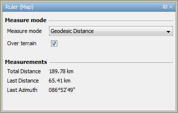
Note that when taking the terrain elevation into account, the geodetic distance of a path may be greater than the rhumbline distance of the path because the geodetic line may cross an elevated area that the rhumbline does not cross.
|
In case the selected terrain data contains unknown or invalid elevation values, the distance over terrain cannot be calculated and the distances are set to Unknown. |
Weather and Environment Standards
After installing the Weather and Environment Standards component, you can load NetCDF, GRIB, and BUFR SIGWX data formats.
Working with NetCDF and GRIB data
Lucy allows you to load NetCDF data and GRIB data.
The NetCDF data format describes array-oriented scientific data. The NetCDF standard itself does not impose any semantic rules or conventions, just like XML files or comma-separated value files. Lucy mainly supports data that complies to the Climate and Forecast (CF) Metadata Conventions and GRIB data.
Refer to the NetCDF documentation for more information.
The GRIdded Binary (GRIB) file format is a standard raster format developed by the World Meteorological Organization (WMO) for meteorological data.
You can use the File→ Open menu to load NetCDF or GRIB data. The layers tree contains layers for the loaded data. To filter the data on one or more of its dimensional ranges, you can make use of sliders displayed on the map. For instance, if you load a file containing zonal current data measured at several water depth levels, you can use a Depth slider to visualize the zonal currents at a particular depth.
Two-dimensional data sets, such as wind or flux, are sometimes stored in two separate files each representing one dimension
or parameter (direction or strength). When loading one of the two files, Lucy will automatically load the related file if
both files are stored in the same directory and have an equal file name (only differing in the parameter value). For example
when opening rlm13_33_0000_100.grb, the file rlm13_34_0000_100.grb is opened as well.
You can change the color of one-dimensional NetCDF or GRIB data, such as pressure or cloud cover, by opening the properties panel and clicking on the Paint style tab as described in The color bar.
Working with WAFS SIGWX data in BUFR format
The Weather and Environment Standards component also includes support for World Area Forecast System (WAFS) Significant Weather (SIGWX) data in BUFR format. WAFS SIGWX files contain information on weather and other environmental phenomena such as clouds, jet streams, and volcanoes. This information is published by the London and Washington World Area Forecast Centres (WAFCs) as SIGWX bulletins and charts, which are used by the aviation community for flight planning.
You can use the File → Open menu to open SIGWX BUFR files in Lucy. The layers tree will contain layers for the types of weather features in the files. The features are visualized to closely match the SIGWX charts produced by WAFS.
For more information on WAFS, WAFCs, and SIGWX, see What is a WAFC? from Met Office UK.
Real-time Engine
After installing the Real-time Engine component, you can load your radar video data, and show the radar video on the map.
|
To find out how to set up such a custom radar video feed for LuciadLightspeed decoding and visualization, see the Radar feeds documentation. If you want to visualize ASTERIX radar video data, make sure that the Radar Connectors component is installed. For more information, see Radar Connectors. |
The visualization shows the radar data as blips in the typical radar circle consisting of a grid, range rings and a rotating sweep line. For an example, see the Radar Video theme in the Lucy Showcase application.
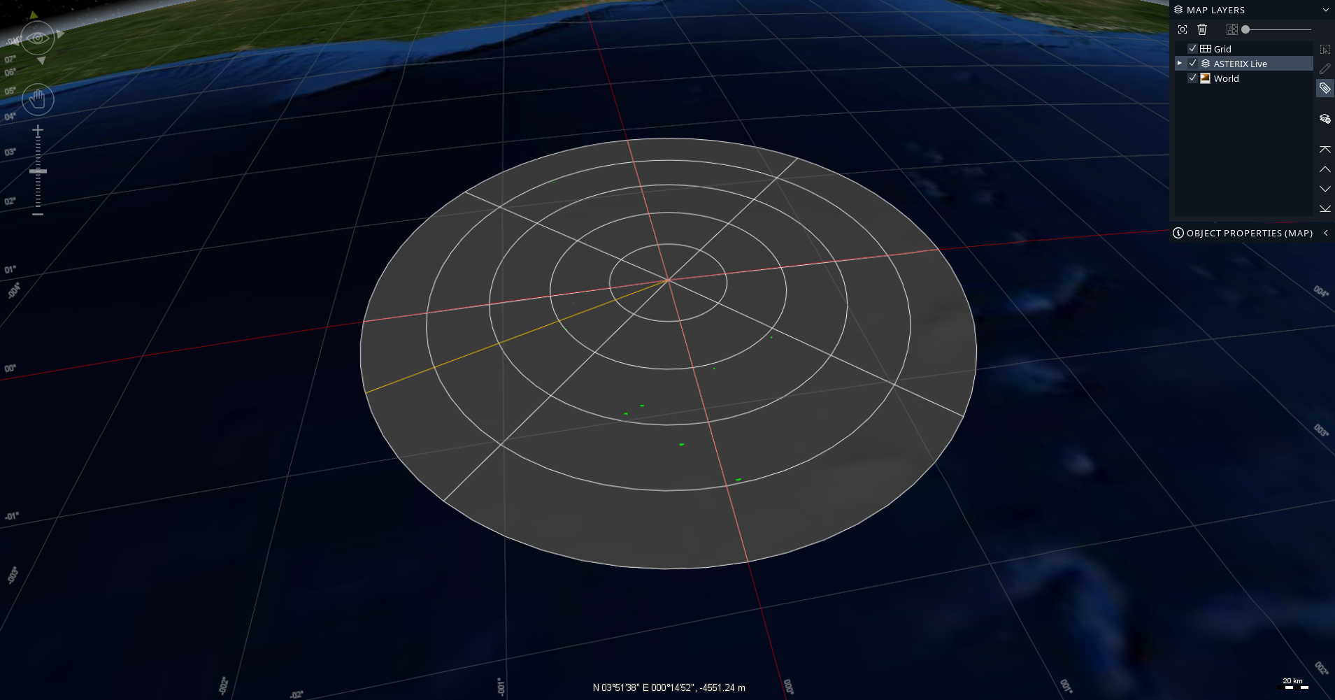
Once your radar video is on-screen, you can change the appearance of the radar circle as well as the blips.
To change the styling of the radar video, open the properties panel of the layer containing the radar video data, and go to the Paint style tab.
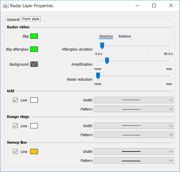
Changing radar blip styling
An object detected by the radar is shown as a blip on the screen. Changing the styling and the display time of such a blip may facilitate the tracking and analysis of radar detections.
The blips are typically brighter if the detected object is large, while smaller object detections are reflected in dimmer blips.
You can change the blip visualization in the following ways:
- Change the blip color
-
Click the Blip color rectangle to choose a different color in the color selector dialog box. For more information, see The color selector.
- Change the blip afterglow to create a trail
-
By default, new blips fade out fairly quickly once the radar sweep line has passed over. To show the blips for a longer time, drag the Afterglow duration slider to the right. You can define the duration time in seconds or number of sweep line revolutions. Click the Relative option over the slider to define the afterglow duration as a revolution number.
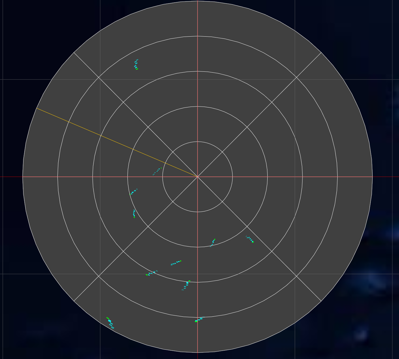 Figure 127. Blip history trails
 - Telling recent and old blips apart
-
In the case of a moving object, a new detection blip will appear at a new position after a full revolution of the sweep line. Depending on the afterglow duration, the previous blip may still be visible. If you want to distinguish those old blips more easily from the most recent blip, you can select a different color for them. Click the Blip afterglow color rectangle to pick another color.
- Increase the color intensity
-
Large objects result in a detection with a high amplitude. Blips for high-amplitude detections will have a more intense color, while blips for small objects will be relatively dim. Increase the color intensity for all blips on the view by dragging the Amplification slider to the right.
- Reduce radar noise
-
Radar noise may lead to many unwanted low-amplitude detections obscuring the relevant blips. To clear up your radar view, you can reduce radar noise by dragging the Noise reduction slider to the right. As a result, the threshold for showing detections as blips will increase.
Changing the radar view
- Change the background color
-
Select the Background color rectangle to set a different background color for the entire radar circle background. For instance, to increase the contrast between the blips and the radar background, after you changed the blip colors.
- Change the grid line styling
-
Change the line color and the line width and pattern of the white radial lines in the Grid section.
- Change the range ring line styling
-
Change the line color and the line width and pattern of the range rings in the Range rings section.
- Change the sweep line styling
-
Change the line color and the line width and pattern of the radar sweep line in the Sweep line section.
Radar Connectors
After installing the Radar Connectors component, you can load ASTERIX data.
Working with ASTERIX data
The All purpose STructured Eurocontrol suRveillance Information eXchange (ASTERIX) format is the standard format for Air Traffic Management (ATM) surveillance data as developed by EUROCONTROL. Note that Lucy does not support all data categories. The LuciadLightspeed Asterix documentation provides more information on the supported data categories and their usage.
After installing the Radar Connectors component, you can load ASTERIX data from a file by using the File→ Open menu, or connect to a radar video stream with File→ Connect To. A new layer is created for the ASTERIX data and added to the layer tree.
To view the loaded data in realtime, select the Tools→ Previewer menu item. The Previewer panel appears in the top left corner of the application window and shows the loaded ASTERIX data sets. You can select one or more data sets for simulation in the map view. Using the Previewer describes the functionality of the Previewer panel in detail. To view the properties of an ASTERIX track, select the track in the map view and open the Object properties panel by double-clicking on the track or selecting Map→ Object Properties. Figure 128, “The Object properties panel of an ASTERIX track” shows the Object properties panel of an ASTERIX track.
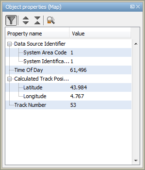
When zooming in on a track in the map view, a label with the track number is added to the track. During a simulation the location
of the tracks and the labels change. The labels automatically reposition to prevent label overlap. In the rare case that labels
overlap, you can select a label and drag and drop it to another location. To turn labeling off, select the corresponding layer
in the layer tree and click on the ![]() icon in the layers toolbar. You can change the label content and style in the layer properties panel as described in The layer properties panel.
icon in the layers toolbar. You can change the label content and style in the layer properties panel as described in The layer properties panel.
Defining ASTERIX radar locations and filters
Most of the Asterix files contain data relative to the location of the radar which captured the data, without specifying the location of the radar itself. If you know the location of the radar you can pass this information to Lucy, which will in turn use the radar location to place the data in the correct location on the map. You can enter the location in the ASTERIX settings dialog, which is opened from Edit→ ASTERIX settings… (see Figure 129, “The ASTERIX settings panel”).
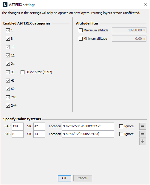
In Specify radar systems, add the SAC and SIC radar identification codes of the data you want to load, and then enter the location coordinates of the radar system with those System Area Code (SAC) and System Identification Code (SIC). Click the + button to identify and locate more radar systems, and the - button to delete a radar system specification.
Furthermore, the Ignore check box in Specify radar systems allows you to mark which radar systems should be included and which ones should be ignored. Lucy will only load the data of the radar systems for which the Ignore check box is not selected. Radar systems that are not specified, are always loaded.
The ASTERIX settings dialog also provides filtering functionality for the loaded Asterix data. You can choose which categories to include from the list of supported ASTERIX categories. Only the selected categories will be loaded. You can also filter out ASTERIX data above a maximum altitude limit and below a minimum altitude limit.
|
Changes made in the ASTERIX settings dialog are only applied to Asterix data that is loaded after the changes have been made. Data that was already loaded remains unaffected. |
The list of categories contains two versions of category 30: the default version and the version '2.5 ter'. The '2.5 ter' version originated in 1997 and is a draft of the category 30 specification. The default category 30 is the final version of this draft (V6.1). Data in the draft version cannot be automatically distinguished from data in the final version, and the two versions are binary incompatible. Therefore, you must explicitly select the version you want to use in the ASTERIX settings dialog, which prevents you from selecting them both at the same time. By default, the final category 30 is selected.
Using the ASTERIX final format
The ASTERIX standard only defines the format for live feeds. It does not define a file format to store recorded feeds. Simply dumping the live feed to a file has its limitations because certain timing information would be missing. Lucy therefore recommends the (unofficial) ASTERIX final file format. The ASTERIX final format is a simple extension of the ASTERIX standard. Each ASTERIX final record is composed like this:
HEADER NormalAsterixBlock1 NormalAsterixBlock2 ... FOOTER
These ASTERIX final records are concatenated in a file, one after the other.
The header of eight bytes is composed like this:
|
byte 0 |
length(msb) |
|
byte 1 |
length(lsb) |
|
byte 2 |
board number |
|
byte 3 |
linenumber |
|
byte 4 |
recording day |
|
byte 5 |
time(msb) |
|
byte 6 |
time |
|
byte 7 |
time(lsb) |
The length is a two byte integer, starting with the most significant byte. It includes the length of the header and the footer itself. The fields board number, line number and recording day are generaaly not used and set to 0. The time is expressed in hundredths of a second past midnight as a three-bytes integer, starting with the most significant byte.
The footer of 4 bytes is composed of 4 times 0xa5 (decimal 165).
Files in the ASTERIX final format typically have the file extension .astfin.
Editing ASTERIX Trajectories
The ASTERIX data model contains a lot of properties. Many of them change with time, like the location or altitude of a track. Other properties, a callsign for instance, are the same for an entire ASTERIX trajectory. In many cases these constant properties have no values, meaning that that information was not available in the feed that was stored. Lucy allows you to fill in missing data for most constant properties using the Table view or the Object properties. It also allows you to delete trajectories you are not interested in, for instance cars that are picked up by the radar.
To edit trajectory properties, first make sure that the corresponding ASTERIX trajectory layer is editable, as explained in Working with layers. Note that you can only edit the properties of an editable layer. You cannot edit the geometry of the trajectories on the map. You can remove selected trajectories, however, by pressing the delete button or by right-clicking the map, and choosing the Delete menu item from the popup menu.
You can also edit ASTERIX properties in the table view and the Object Properties panel. To edit constant ASTERIX properties in a table, open the table view for a trajectory layer. If you move the mouse over the table, the table cells that can be edited will be highlighted. To edit properties in the Object Properties panel: double-click on a trajectory to access the properties in the panel, and move the mouse over the second column. Again, editable cells will be highlighted.
If you click on an editable cell, a text cursor will allow you to type the value. Certain constraints apply: a call sign can only contain ASCII[1] characters, for instance, and has a maximum length of 7. Some other properties use the smaller IA5[2] character set. If the typed text does not comply with the constraints, the background of the cell will turn red. For more information about what values are acceptable for the various properties, see Value constraints for editable properties.
If a property accepts a limited number of possible values, a combo box will appear instead of a text cursor. The combo box allows you to choose a value from a list of options.
Note that you can also change the constant properties for a track layer in the table view, or in the Object properties panel for a selected track. Track changes will automatically be applied on the entire trajectory.
Value constraints for editable properties
For category 10 tracks:
-
TargetIdentification | TargetIdentification: IA5, max 8 characters.
-
TargetIdentification | STI: choose from list of options.
For category 11 trajectories:
-
TargetIdentification | TargetIdentification: IA5, max 8 characters.
-
TargetIdentification | STI: choose from list of options.
-
Callsign: ASCII, max 7 characters
-
IFPS_FLIGHT_ID | FlightNumberType : choose from list of options
-
IFPS_FLIGHT_ID | FlightNumber : integer between 0 and 134217727.
-
FlightCategory | GeneralOrOperationalAirTraffic : choose from list of options
-
FlightCategory | FlightRulesType : choose from list of options
-
FlightCategory | RVSM : choose from list of options
-
FlightCategory | HighPriorityFlightType : choose from list of options
-
TypeOfAircraft: ASCII, max 4 characters
-
WakeTurbulenceCategory: ASCII, max 1 character
-
DepartureAirport: ASCII, max 4 characters
-
DestinationAirport: ASCII, max 4 characters
For category 11 tracks:
-
TargetIdentification | TargetIdentification: IA5, max 8 characters.
-
TargetIdentification | STI: choose from list of options.
-
FlightPlanRelatedData | Callsign: ASCII, max 7 characters
-
FlightPlanRelatedData | IFPS_FLIGHT_ID | FlightNumberType : choose from list of options
-
FlightPlanRelatedData | IFPS_FLIGHT_ID | FlightNumber : integer between 0 and 134217727.
-
FlightPlanRelatedData | FlightCategory | GeneralOrOperationalAirTraffic : choose from list of options
-
FlightPlanRelatedData | FlightCategory | FlightRulesType : choose from list of options
-
FlightPlanRelatedData | FlightCategory | RVSM : choose from list of options
-
FlightPlanRelatedData | FlightCategory | HighPriorityFlightType : choose from list of options
-
FlightPlanRelatedData | TypeOfAircraft: ASCII, max 4 characters
-
FlightPlanRelatedData | WakeTurbulenceCategory: ASCII, max 1 character
-
FlightPlanRelatedData | DepartureAirport: ASCII, max 4 characters
-
FlightPlanRelatedData | DestinationAirport: ASCII, max 4 characters
For category 21 tracks and trajectories:
-
EmitterCategory: choose from list of options.
-
TargetIdentification: IA5, max 8 characters.
For category 30 and 30v2.5 ter tracks and trajectories:
-
CallSign: ASCII, max 7 characters.
-
PLNNumber: integer between 0 and 65535.
-
DepartureAirport: ASCII, max 4 characters
-
DestinationAirport: ASCII, max 4 characters
-
CategoryOfTurbulence: ASCII, max 1 character
-
TypeOfAircraft: ASCII, max 4 characters.
-
FlightCategory | SubCategory: integer between 0 and 7, can’t be empty.
-
FlightCategory | GeneralAirTrafficVsOperationalAirTraffic: choose from list of options.
-
FlightCategory | FlightRules: choose from list of options.
For category 48 tracks and trajectories:
-
AircraftIdentification: IA5, max 8 characters.
For category 62 trajectories:
-
TargetIdentification | TargetIdentification: IA5, max 8 characters.
-
TargetIdentification | STI: choose from list of options.
-
Callsign: ASCII, max 7 characters
-
IFPSFlightId | Type : choose from list of options
-
IFPSFlightId | Number : integer between 0 and 134217727.
-
FlightCategory | GeneralVsOperationalAirTraffic : choose from list of options
-
FlightCategory | FlightRules : choose from list of options
-
FlightCategory | RVSM : choose from list of options
-
FlightCategory | Priority : choose from list of options
-
TypeOfAircraft: ASCII, max 4 characters
-
WakeTurbulenceCategory: ASCII, max 1 character
-
DepartureAirport: ASCII, max 4 characters
-
DestinationAirport: ASCII, max 4 characters
For category 62 tracks:
-
TargetIdentification | TargetIdentification: IA5, max 8 characters.
-
TargetIdentification | STI: choose from list of options.
-
FlightPlanRelatedData | Callsign: ASCII, max 7 characters
-
FlightPlanRelatedData | IFPSFlightId | Type : choose from list of options
-
FlightPlanRelatedData | IFPSFlightId | Number : integer between 0 and 134217727.
-
FlightPlanRelatedData | FlightCategory | GeneralVsOperationalAirTraffic : choose from list of options
-
FlightPlanRelatedData | FlightCategory | FlightRules : choose from list of options
-
FlightPlanRelatedData | FlightCategory | RVSM : choose from list of options
-
FlightPlanRelatedData | FlightCategory | Priority : choose from list of options
-
FlightPlanRelatedData | TypeOfAircraft: ASCII, max 4 characters
-
FlightPlanRelatedData | WakeTurbulenceCategory: ASCII, max 1 character
-
FlightPlanRelatedData | DepartureAirport: ASCII, max 4 characters
-
FlightPlanRelatedData | DestinationAirport: ASCII, max 4 characters
For category 244 tracks and trajectories:
-
TargetIdentification: IA5, max 8 characters.
-
AircraftType: ASCII, max 4 characters.
-
ADSBEmitterCategory: choose from list of options.
Saving ASTERIX Data
You can save your changes you made to ASTERIX trajectories by using the menu items Save and Save As… in the File menu. If the destination filename ends with .astfin, the ASTERIX data is stored in Using the ASTERIX final format. Otherwise the data is saved in the raw ASTERIX format.
Note that you can only save original ASTERIX layers this way. You cannot save trajectories you drew yourself as an ASTERIX file, for instance.
Aviation Standards
After installing the Aviation Standards component, you can load aeronautical data, including the AIXM, ARINC, and DAFIF formats.
Working with Aeronautical Information Services (AIS) data
You can view the properties and edit the aircraft performance settings (APS) of terminal procedures provided by an AIXM, ARINC, or DAFIF dataset. The associated geometry and APS determine how the procedure is visualized.
Viewing terminal procedure properties
To view the properties of a terminal procedure, select the procedure on the map, right-click and select Properties to open the Object properties panel. The AIS Procedure Trajectories tab in this panel shows the details of the procedure’s trajectories, as illustrated by Figure 130, “The AIS Procedure Trajectories tab of the procedure properties panel”.
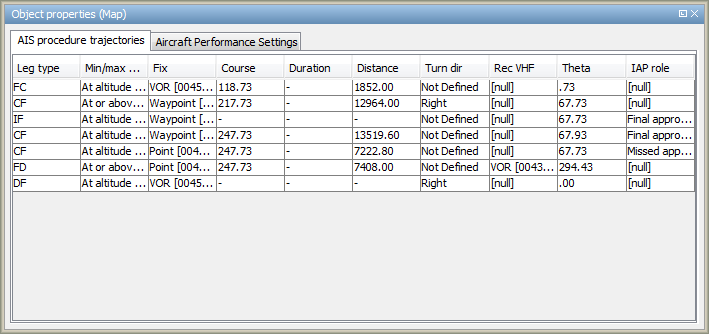
See Changing the APS settings of terminal procedures for more information about the Aircraft Performance Settings tab.
Changing the APS settings of terminal procedures
Once the aeronautical data has been loaded, you can edit the APS of one or more procedures and view the resulting visualization in real-time.
You can change the following APS settings:
-
Minimal turn radius
-
Climb rate
-
Descent rate
-
Default holding length
-
Holding radius
-
Manual termination distance
-
Default speed
-
Procedure turn radius
You can change the APS of just one procedure, or of all procedures:
-
To change one procedure: select a procedure on the map, right-click and select Properties to open the Object properties panel of the procedure. Change the APS for the selected procedure in the Aircraft Performance Settings tab of the panel, by using the Editor sliders, or by selecting and applying a set of pre-defined APS settings. For a description of the AIS procedure trajectories panel, see Viewing terminal procedure properties.
-
To change all procedures that are loaded in the current map: select Tools→ Procedures→ Set default aircraft performance. Use the Editor sliders to change the settings individually, and click the Apply to all procedures button to apply the changes. This panel offers the possibility to select another preset, open a file with other settings, and save the changed settings to file.
|
The changed settings apply to the procedure immediately and that the changes are visualized in real-time. |
Working with AIXM data
The Aeronautical Information Exchange Model (AIXM) file format is an XML-based format originally developed by Eurocontrol. The AIXM 5.1 format is developed by Eurocontrol and the United States Federal Aviation Administration (FAA). The AIXM file format is used for aeronautical data such as airspaces, routes, and navaids. LuciadLightspeed offers support for AIXM versions 3.3, 4.0, 4.5, and 5.1. Time-dependent data in the AIXM 5.1 format can be simulated in realtime.
The AIXM 3 and 4 formats
After installing the Aviation Standards component, you can load AIXM data for versions 3 and 4 by using the File→ Open menu. It is possible to select either snapshot data, data that has not been loaded before, or update data, updates to data that has already been loaded. If you select an AIXM file with snapshot data, a dialog box allows you to select the objects that you want to load, as shown in Figure 131, “The dialog box for selecting AIXM objects”. To load all AIXM object types, select the Select all check box first.
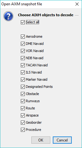
If you select an AIXM file with updates, a dialog box allows you to select the loaded layers that need to be updated, as shown in Figure 132, “The dialog box for updating AIXM layers”.
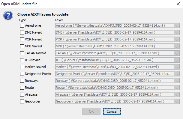
The loaded data is displayed in the map view, and the corresponding layers are added to the layer tree.
In Lucy GXY, the Map→ Colors→ AIXM 3/4 menu item is added. It allows you to change the colors of the displayed AIXM data.
|
The Aviation Standards component provides functionality to view and edit the aircraft performance settings of a loaded procedure as described in Working with Aeronautical Information Services (AIS) data. |
The AIXM 5.1 format
After installing the Aviation Standards component, you can load AIXM 5.1 data by using the File→ Open menu. The loaded data is displayed in the map view and the corresponding layers are added to the layer tree. Each of the objects (or features) of the loaded AIXM 5.1 data set are represented in a separate layer, also the objects that are not displayed in the map view.
To edit an AIXM 5.1 geometric object, first make the layer editable by selecting it in the layer tree, right-clicking, and selecting Editable from the menu that appears. You can then select an AIXM 5.1 geometric object on the map and drag it to change its properties. Save the changes to the layer by selecting the File→ Save As menu item.
To view the properties of an AIXM 5.1 geometric object, select the object on the map, right-click and select Properties. The Object properties panel appears in the top left corner of the application window. The properties tree follows the XML structure of the selected object and allows you to view the available properties or all properties of the object.
AIXM 5.1 objects such as airspaces or navaids consist of time slices whereby each time slice contains the object properties that are valid for that time period. To view the properties of an AIXM 5.1 layer including the time slices you need to display the layer properties in table format as described in Displaying your data in a table view.
Working with ARINC data
The Aeronautical Radio Incorporated (ARINC) format is the standard format for aeronautical data such as airspaces, routes, and navaids. It is mainly used in civilian applications. Lucy supports version 15, 17, and 18 of the ARINC 424 specification.
After installing the Aviation Standards component, you can load ARINC data by using the File→ Open menu. When you select an ARINC file, a dialog box allows you to select the objects that you want to load, as shown in Figure 133, “The dialog box for selecting ARINC objects”. To load all ARINC object types, select the Select all check box first.
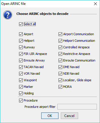
To restrict the loading of procedures to one or more airports, enter a comma-separated list of airport identifiers (as defined by the ICAO) in the box under Procedure airport filter. Enter for example, KALB, KART, KBUF, KHPN, KIAG, KISP, KJFK, KLGA, KMSS, KOGS, KROC, KSWF, KSYR to view the airports located in the New York area.
The loaded data is displayed in the map view, and the corresponding layers are added to the layer tree.
In Lucy GXY, the Map→ Colors→ ARINC menu item is added. It allows you to change the colors of the displayed ARINC data.
|
The Aviation Standards component provides functionality to view and edit the aircraft performance settings of a loaded procedure as described in Working with Aeronautical Information Services (AIS) data. |
Working with DAFIF data
The Digital Aeronautical Flight Information File (DAFIF) format is the standard format for aeronautical data such as airspaces, routes, and navaids. It is mainly used in military applications. Lucy supports DAFIF Edition 7 and 8 data.
You can load DAFIF data by using the File→ Open menu. The layers tree contains layers for the loaded DAFIF data.
|
The Aviation Standards component provides functionality to view and edit the aircraft performance settings of a loaded procedure as described in Working with Aeronautical Information Services (AIS) data. |
Defense Standards
After installing the Defense Standards component, you can load the VPF and MGCP formats.
Working with VPF data
The Vector Product Format (VPF) is a file format used for large geographic databases that are based on a georelational data model. The supported file formats are based on and are compatible with the following standards:
-
VPF: MIL-STD-2407, 28 June 1996
-
GeoSym: MIL-DTL-89045, 17 June 2004
After installing the Defense Standards component, you can load individual VPF databases using the File→ Open menu.
Loading VPF data in Lucy
When you load a .dht or .lat file, the database structure is displayed as map layers organized in a layer tree.
If you do not see the data on the map, fit the map to the data, and start zooming in to make the data visible.
Figure 134, “A selection of VPF data with the corresponding layer tree” shows a selection of VPF data in the map view and the corresponding VPF panel and layer tree.
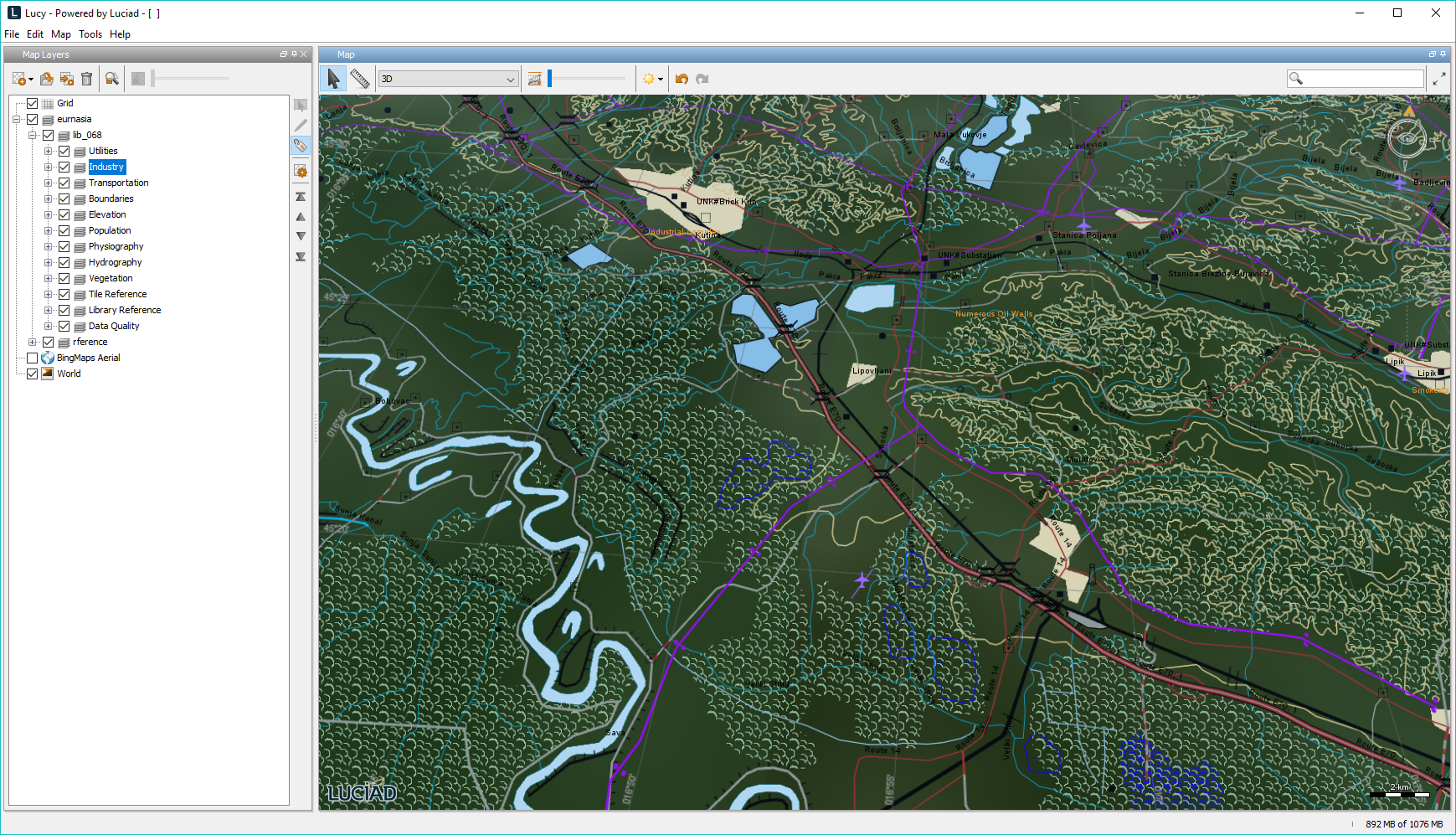
Loading VPF data in Lucy GXY
When you load a .dht or .lat file, the VPF panel appears in the top left corner of the application window showing the loaded database in a tree structure.
To display individual coverages and feature classes in the map view, select the corresponding check boxes and click on the Update button under the data tree. The corresponding data layers are added to the layer tree in the Map layers panel, and the map shows the selected data.
If you do not see the data, and the corresponding layer is grayed out in the layer tree, fit the map to the data, and zoom in.
|
When you close the VPF panel, the data is no longer displayed and the data layers are removed from the layer tree. |
To load multiple databases, select the Map→ Data→ VPF Browser menu item. Click on the Open database icon![]() top left in the VPF panel. The Set VPF root dialog box appears that allows you to browse to and select the common parent directory of the databases that you want to
load. After selecting the parent directory, click on the Set VPF root button next to the File name box. The subdirectories of the selected root directory will automatically be scanned and the
databases in all directories will be loaded. The coverages of all loaded databases will be merged, irrespective of their level
of detail (for example VMAP levels 0, 1, and 2). The VPF panel shows the union of coverages as if they are part of one VPF
data set.
top left in the VPF panel. The Set VPF root dialog box appears that allows you to browse to and select the common parent directory of the databases that you want to
load. After selecting the parent directory, click on the Set VPF root button next to the File name box. The subdirectories of the selected root directory will automatically be scanned and the
databases in all directories will be loaded. The coverages of all loaded databases will be merged, irrespective of their level
of detail (for example VMAP levels 0, 1, and 2). The VPF panel shows the union of coverages as if they are part of one VPF
data set.
To limit the display area in the map view to the active Area of Interest, select the corresponding check box in the Options section of the VPF panel.
Symbols help you recognize what kind of data you are seeing. Therefore, Lucy GXY visualizes the VPF data according to the GeoSym symbology set standard. To remove the symbology from your map, de-select the GeoSym check box.
Working with MGCP data
The Multinational Geospatial Co-production Program (MGCP) portrayal standard was developed by the Multinational Geospatial Co-production Program - Technical Group (MGCP-TG). Ultimately, its goal is to allow vendors and producers to portray MGCP data within a Technical Reference Documentation, Version 4 (TRD4) schema on a hardcopy 1:50,000 or 1:100,000 topographic map.
The standard provides symbol rules that associate geospatial feature/attribute data instances from the MGCP Feature Catalogue with agreed symbol specifications. It also provides supplementary non-MGCP feature content and associated agreed symbol specifications required to produce a topographic map.
Loading MGCP data in Lucy
After installing the Defense Standards component, you can use the File→ Open menu to load and display MGCP XML files, which contain the metadata for the MGCP data set. Such an .xml file contains references to .shp files that each contain one feature class for a particular 1-degree-by-1-degree map cell.
In the Choose a format: dialog, select MGCP, and click OK.
The result of loading such an XML metadata file is one layer, named after the file. The layer visualizes all MGCP features for one map cell. As you zoom in on the cell, more and more features become visible. You can select individual features to inspect their properties in the Object Properties panel.
|
If you do not see the data on the map, start zooming in to make the MGCP features visible. |
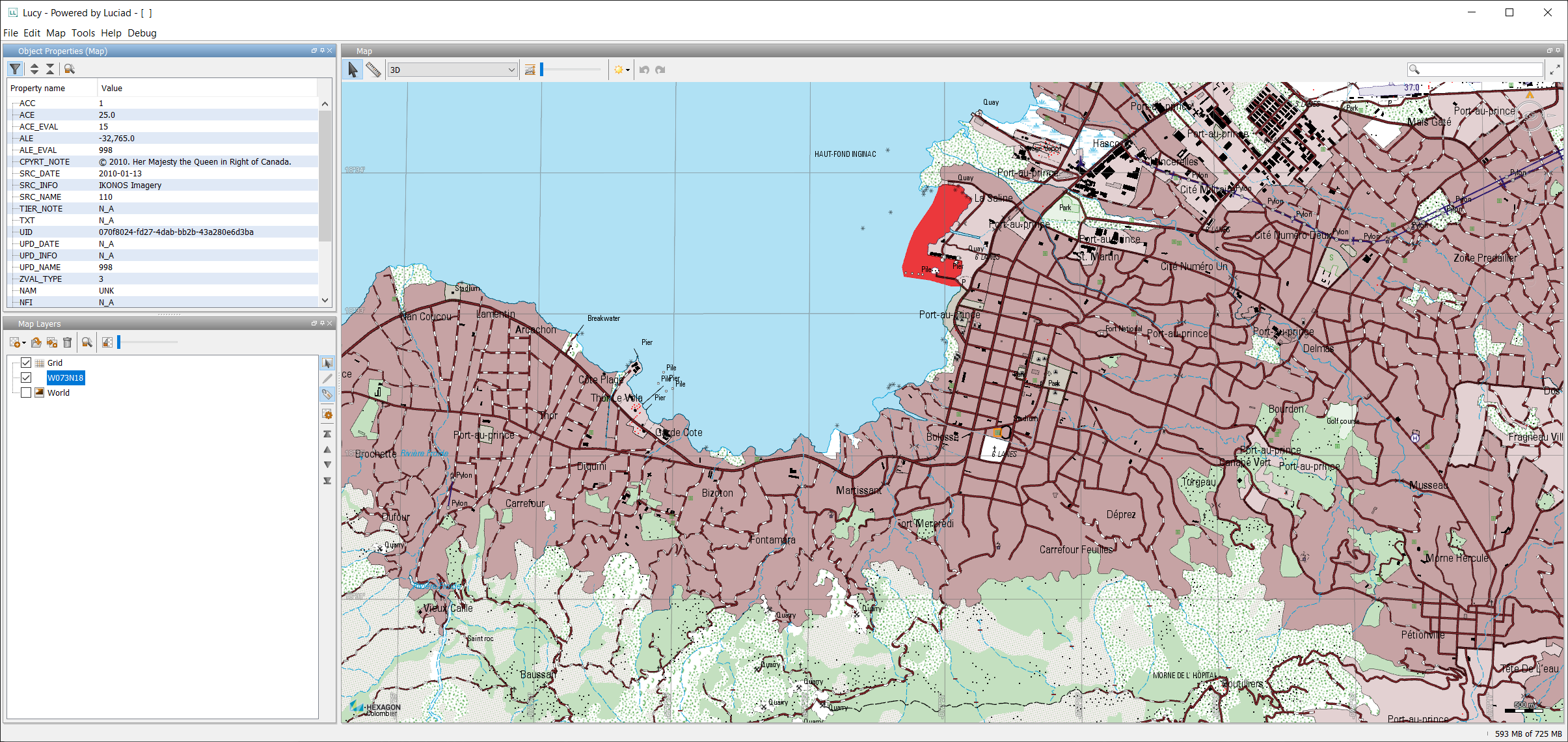
Defense Symbology
The Defense Symbology component offers support for the symbol sets as defined by the following military standards:
-
MIL-STD 2525d, developed by the United States Department of Defense (DoD)
-
APP-6D, developed by the North Atlantic Treaty Organization (NATO)
These standards provide guidelines and criteria for the development and display of Command, Control, Communications, Computers, and Intelligence (C4I) warrior symbology. The standards are very similar and have many symbols in common.
In addition, the Defense Symbology component allows you to load NVG data.
You also need the Defense Symbology component to add an MGRS grid to the map view.
Creating a layer for military symbols
After you installed the Defense Symbology component, you can create a military symbology layer, and start adding either MS2525 or APP-6 military symbols.
You can create a military symbology layer in two ways:
-
Click the Add layer icon
, and select the appropriate symbology type from the drop-down list: MS2525d or APP6D.
-
Select The File→ New→ Layer menu item, select the appropriate symbology type from the dialog, and click OK.
After you select a symbology standard for your layer, the corresponding layer is added to the layer tree and a toolbar appears under the map view. Figure 136, “The symbology toolbar” shows a symbology toolbar.

The icons and menus on the format bar offer the following functionality:
-
The first icon
allows you to add extra layer to the layer tree. You can add a drawing layer or other military symbology layers. For more
information about drawing layers, see Drawing shapes on the map.
-
The search box allows you to search for a military symbol by typing in its name. You can type in any part of the name. As you type, a selection menu will display a list of names containing the text you are typing. To select a symbol, click the appropriate item in the name list. You can now draw the selected symbol on the map. For more information, see Drawing military symbols.
-
The Browse button next to the search box allows you to select symbols from the symbol hierarchy. The symbol hierarchy allows you to drill down into the symbol collection by expanding the various symbol categories. Browse through the categories to find the symbol you want, select it, and click Create. Click on the map to draw the symbol.
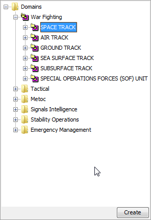
-
The Favorites section in the drawing toolbar displays preferred symbols, for easy access to symbols you draw often. You can change the symbols displayed in this section easily by marking other symbols as your favorite. For more information, see Working with favorite symbols.
- Map-centric Lucy
-
To start drawing military symbols in map-centric Lucy, click the Create military symbols and graphics icon, located in the lower half of the side tool bar.
Drawing military symbols
To add a military symbol to the map:
-
Type a search term in the Search box of the symbology tool bar, until the Search box menu lists the symbol you are looking for.
-Or-
Click the Browse button next to the search box to browse through the symbol categories and find the right symbol. -
Select the symbol. The cursor changes into a cross.
-
Move the cross cursor to the required location on the map, click the location, and start drawing the symbol.
-
Keep clicking the map to specify all the symbol’s anchor points. When all the required points have been specified and the symbol is complete, the cursor changes into an arrow again. If your symbol does not have a specific number of anchor points, right-click the last anchor point to finish drawing the symbol.
To specify the symbol in detail, open its Object Properties panel. For more information, see Updating the symbol properties.
Updating a symbol
You can update the general properties of a symbol, replace it with a different symbol, or change its location and shape on the map.
Updating the symbol properties
To edit the properties of a symbol, like its affiliation or status, open the Object properties panel by double-clicking the symbol on the map, or by right-clicking the symbol and selecting Properties.
To set the properties, you either select predefined settings from a dropdown menu, or fill in text in a text field.
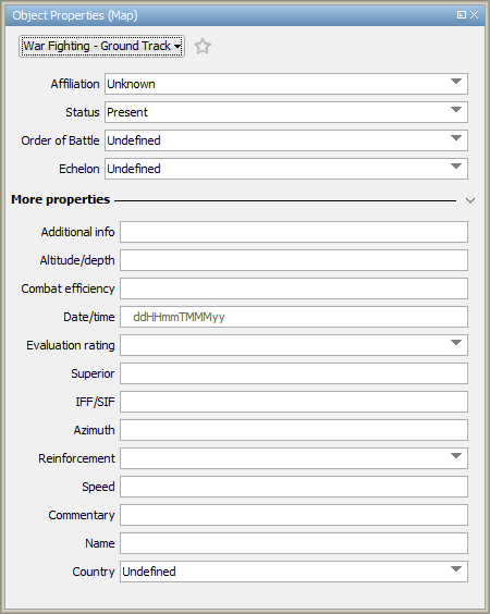
To add more information about the symbol, expand the More properties section in the Object properties panel. The More properties section displays the extra properties available for the selected symbol.
Replacing the symbol
To change the symbol to another one, open its Object Properties panel, and enter a different symbol. You can specify a different symbol by clicking the symbol name at the top of the panel, and finding the new symbol in the symbol hierarchy dropdown menu. Click Select to replace the symbol on the map with the selected symbol.
Moving or reshaping the symbol
To change a symbol’s location or shape on the map, click the symbol to select it. To move the symbol, drag it across the map to its new location. To change the shape of the symbol, hover over one of the shape’s editing points until the cursor changes to a cross, and then drag the editing points until the symbol has the required shape.
Working with favorite symbols
The Favorites section in the symbology toolbar allows you to quickly add symbols to the map, without having to search for them first.
You can customize the Favorites section according to your preferences, by adding and removing symbols.
To add a symbol to the Favorites, first find and draw it on the map. Then open the Object properties panel and select the Star icon next to the symbol name.
To remove a symbol from the Favorites, right-click it in the toolbar, and click Remove. You can also open the Object properties panel for a symbol you drew, and deselect the Star icon next to the symbol name.
Your favorite symbol choices are preserved between Lucy restarts. When you restart the Lucy application, the symbology toolbar will display the same favorites as it did in the previous session.
Working with NVG data
NATO Vector Graphics (NVG) allow NATO members to exchange situational awareness information, and construct a Common Operational Picture (COP). NVG data consists of military symbols, shapes, and text. After installing the Defense Symbology component, you can use the File→ Open menu to load and visualize a file with NVG military symbols and shapes on the map.
See the NVG developer documentation for more information about the LuciadLightspeed support for NVG.
Maritime Standards
After installing the Maritime Standards component, you can load ECDIS S-57 and S-101 data, with appropriate visualization defined by the S-52 and S-101 standards respectively.
Lucy supports ENC, IENC and AML.
Working with ECDIS data
Lucy provides support for loading and displaying hydrographic data that complies with the S-101, S-57 and S-52 standards as published by the International Hydrographic Organization (IHO). Such data is used in Electronic Chart Display Information Systems (ECDIS).
After installing the Maritime Standards component, you can use the File→ Open menu to load:
-
Individual Electronic Navigation Chart (ENC) cell files with extension .000.
Lucy loads updates, which have extensions like .001, .002, and so on, automatically with the .000 file. It is not possible to load them separately. -
Catalog files, with extension .031 for S-57 and .xml for S-101.
Because Lucy uses lazy loading when reading catalogs, it supports the use of large datasets. Depending on the available data and the current map scale, different levels may be used to represent different map areas.
Setting the display style for S-57 data
When S-57 data is loaded on the map, the S52 Style or AML Style panel allows you to change the style settings of all loaded S-57 data. Expand the Text and Advanced sections to see all the fields:
|
Field |
Use |
|
Basic: Color scheme |
Choose the color scheme that best reflects the time of day: bright daytime colors, or darker dusk or nighttime colors. |
|
Basic: Display category |
Select how much of the data is visible on the map. The available options filter out map objects based on an S-52 symbology categorization. To see only a basic amount of data, choose Display Base. To see the standard amount of data, choose Standard. Choose Other to see even more objects, and to make your own selection of visible object classes. To filter out object classes, choose the Filter button that appears next to the Other button when it is clicked. |
|
Safety: Depth areas |
Indicate how you want the depth safety areas for a ship to be displayed on the map, based on the ship’s safety contour. Click Two shades to distinguish between unsafe and safe depth areas. Two shades of blue are used to mark the areas. The boundary between the safe and unsafe areas is demarcated with a dark line. You can modify a ship’s safety contour by entering a different value in the Safety contour field in meters. As a result, safe and unsafe depth areas may shrink or expand. Choose Four shades to add distinctions within the unsafe and safe depth areas. These distinctions are based on the ship’s shallow and deep contours, indicated in meters. You can enter other shallow and deep contours in the appropriate text fields. |
|
Safety: Isolated dangers in unsafe water |
Select this check box to display isolated dangers, like rocks, in unsafe depth areas, even though the ship is not allowed to enter these areas. |
|
Safety: Unsafe water hatching |
If you do not want to rely on a color scheme alone, select this check box to display an additional hatch pattern in unsafe depth areas. |
|
Safety: Depth soundings |
Select this check box to display depth sounding values on the map. To see the values, zoom in closely. Depth measurements are displayed in a darker color in unsafe depth areas. |
|
Safety: Ship beam and Ship air draft |
Configure your ship’s width and height above water, in meters. This setting only has effect on InlandECDIS (IENC) datasets: it is used for displaying bridge safety. |
|
Text: Show text |
Select this check box to display the names of objects on the map. Use this option with care, because it may clutter the map. |
|
Text: Abbreviate text |
Select this check box to allow the use of abbreviations in displayed text. Currently, only Nature-of-Surface (NATSUR) attributes are abbreviated. |
|
Text: Language |
To use the international name for an object in displayed text, select International. To use a local name, select National. |
|
Advanced: Boundaries |
Select Plain to use only solid and dashed lines to display boundaries. Select Symbolized to use more distinctive and informative symbols to display boundaries. |
|
Advanced: Icons |
Select Simplified if you just want to see distinctive screen icons. If you want more detailed icons, which are more suitable for printing, select Paper chart. |
|
Advanced: Light sector lines |
Select Short to display light sector lines with a fixed length. Select Real length if you want to display the lines with the actual light visibility distance. |
|
Advanced: Navigational purpose boundaries |
Select this check box if you want to display a solid border between catalogue cells with different navigational purposes. |
|
Advanced: Overzoom hatching |
Select this check box to display a hatching pattern in catalogue cells if you zoom in beyond the intended viewing level of a catalogue cell. |
|
Advanced: Cell outlines |
Displays the outlines of catalogue cells if you have not yet zoomed in to an appropriate level for viewing the cell. This setting is not a part of the S-52 specification. |
|
Advanced: Land areas |
Select this check box to display land areas and built-up areas. Deselect the check box if you want to hide those land areas, and display other data in those locations instead, such as imagery. |
|
Advanced: Metadata |
Select this check box to display metadata on the map, such as information about the data quality. To see the metadata, first select the Other option in the Basic: Display category section. |
|
The S-63 component adds support for loading S-63 datasets, which are encrypted S-57 datasets. Note that Lucy can only load S-63 data sets for which you have specified an S-63 User Permit in the license file. The LuciadLightspeed ECDIS documentation provides more information about using the S-63 component. |
Setting the display style for S-101 data
Similarly, when S-101 data is loaded on the map, the S101 Style panel allows you to change the style settings of all loaded S-101 data. Expand the Advanced section to see all the fields:
|
Field |
Use |
|
Basic: Color palette |
Choose the color palette that best reflects the time of day: bright daytime colors, or darker dusk or nighttime colors. |
|
Basic: Display mode |
Select how much of the data is visible on the map. The available options filter out map objects based on an S-101 symbology categorization. To see only a basic amount of data, choose Display Base. To see the standard amount of data, choose Standard. Choose Other to see even more objects. |
|
Safety: Depth areas |
Indicate how you want the depth safety areas for a ship to be displayed on the map, based on the ship’s safety contour. Click Two shades to distinguish between unsafe and safe depth areas. Two shades of blue are used to mark the areas. The boundary between the safe and unsafe areas is demarcated with a dark line. You can modify a ship’s safety contour by entering a different value in the Safety contour field in meters. As a result, safe and unsafe depth areas may shrink or expand. Choose Four shades to add distinctions within the unsafe and safe depth areas. These distinctions are based on the ship’s shallow and deep contours, indicated in meters. You can enter other shallow and deep contours in the appropriate text fields. |
|
Safety: Isolated dangers in unsafe water |
Select this check box to display isolated dangers, like rocks, in unsafe depth areas, even though the ship is not allowed to enter these areas. |
|
Advanced: Boundaries |
Select Plain to use only solid and dashed lines to display boundaries. Select Symbolized to use more distinctive and informative symbols to display boundaries. |
|
Advanced: Icons |
Select Simplified if you just want to see distinctive screen icons. If you want more detailed icons, which are more suitable for printing, select Paper chart. |
|
Advanced: Light sector lines |
Select Short to display light sector lines with a fixed length. Select Real length if you want to display the lines with the actual light visibility distance. |
|
Advanced: Overzoom hatching |
Select this check box to display a hatching pattern in catalogue cells if you zoom in beyond the intended viewing level of a catalogue cell. |
|
Advanced: Cell outlines |
Displays the outlines of catalogue cells if you have not yet zoomed in to an appropriate level for viewing the cell. |
|
Advanced: Ignore minimum scale |
Select this check box to ignore the minimum scale for objects to be visible. This ensures that all objects are visible at all zoom levels. |
Appendix A: Supported data formats
Table 3, “Supported data formats” shows the data formats and corresponding file extensions that Lucy supports. Refer to Appendix B, Acronyms and abbreviations for definitions of the acronyms and abbreviations. To add support for some of these data formats, you need to install optional components first.
|
File type |
File name/extension |
Component |
Comments |
|
ACE2 |
.ace2, .ace2.gz |
Advanced Raster Connectors |
ACE2 Global Elevation Model. |
|
AIXM |
.xml |
Aviation Standards |
See Working with AIXM data. Also requires AIS component. |
|
APP-6C |
.ims |
Defense Symbology |
See Defense Symbology. |
|
ARINC |
.txt, .pc, FAA*, .ari |
Aviation Standards |
|
|
ArcInfo ASCII Grid Format |
.asc, .grd |
LuciadLightspeed Essential |
|
|
ArcInfo Binary Grid Format |
.adf |
Advanced Raster Connectors |
|
|
ArcInfo Export Grid Format |
.e00 |
Advanced Raster Connectors |
|
|
ASTERIX |
.asterix |
Radar Connectors |
|
|
Azure Maps imagery |
N/A |
LuciadLightspeed Essential |
|
|
BCI |
.matrxmap |
Defense Standards |
|
|
BIL |
.bil |
LuciadLightspeed Essential |
|
|
Bing Maps imagery |
N/A |
LuciadLightspeed Essential |
|
|
BLX |
.blx, .xlb |
Advanced Raster Connectors |
Magellan BLX Topo. |
|
BSB |
.kap |
Advanced Raster Connectors |
BSB Nautical Chart |
|
BUFR SIGWX |
.bufr, .bin |
Weather and Environment Standards |
|
|
CADRG |
.toc |
Defense Standards |
|
|
CGM |
.cg, .cgm.gz, .cgm.zip |
LuciadLightspeed Essential |
Draped as texture on Lightspeed map. |
|
Collada |
.dae |
LuciadLightspeed Essential |
Embedded in KML files. |
|
DAFIF |
.toc |
Aviation Standards |
|
|
DEM |
.dem, .dem.gz, .dem.zip |
LuciadLightspeed Essential |
|
|
DGN |
.dgn |
Infrastructure Standards |
Adds support for the Bentley Microstation DGN format. |
|
DIMAP |
.dim |
Advanced Raster Connectors |
Adds support for both volume files and data files. |
|
DOQ |
.doq |
Advanced Raster Connectors |
First Generation and New Labelled USGS DOQ. |
|
DMED |
.dmed |
LuciadLightspeed Essential |
|
|
Drawing |
.drawing |
LuciadLightspeed Essential |
Lucy drawing files. |
|
DTED |
.dt0, dt1, dt2 |
LuciadLightspeed Essential |
|
|
DWG |
.dwg, .dxf |
Infrastructure Standards |
Adds support for AutoCAD DWG and DXF versions R13C3, R14, R2000, and R2004. |
|
E57 |
.e57 |
LuciadLightspeed Essential |
See Loading LIDAR data. |
|
Earth terrain repository |
tilerepository.cfg |
LuciadLightspeed Essential |
|
|
ECDIS/S-63 |
.000, .031 |
Aviation Standards/S63 |
See Working with ECDIS data. Draped as texture on Lightspeed maps. |
|
ECRG |
TOC.xml |
Defense Standards |
|
|
ECW |
.ecw |
Advanced Raster Connectors |
|
|
ENVI Header |
.hdr |
Advanced Raster Connectors |
ENVI .hdr Labelled Raster |
|
ERDAS |
.img |
Advanced Raster Connectors |
ERDAS Imagine |
|
ETOPO |
.ETOPO2.raw.bin, ETOPO2v2_MSB.raw, ETOPO5.DAT |
LuciadLightspeed Essential |
|
|
GDAL Virtual |
.vrt |
Advanced Raster Connectors |
|
|
GeoJson |
.json |
LuciadLightspeed Essential |
|
|
GeoPackage |
.gpkg |
LuciadLightspeed Essential |
OGC format for mobile geospatial data |
|
Geospatial PDF |
|
Advanced Raster Connectors |
|
|
GeoSpot |
.dsc, .rep |
Advanced Raster Connectors |
|
|
GeoTIFF |
.tif, .tiff |
LuciadLightspeed Essential |
|
|
GML |
.gml32, .gml31, .gml3, .gml, .xml |
LuciadLightspeed Essential |
|
|
GRIB |
.grb, *.grib, *.dat, *.grb2, *.grib2 |
Weather and Environment Standards |
|
|
GTX |
.gtx |
Advanced Raster Connectors |
NOAA .gtx vertical datum shift. |
|
GXF |
.gxf |
Advanced Raster Connectors |
Grid eXchange File. |
|
HDF5 |
*.hdf, *.h5, *.he5, *.hdf5 |
Weather and Environment Standards |
|
|
HFT |
.hft |
Advanced Raster Connectors |
HF2 heightfield raster |
|
HGT |
.hgt |
Advanced Raster Connectors |
SRTM HGT. |
|
IFC |
.ifc |
Infrastructure Standards |
Adds support for versions 2x3 and 4. |
|
JAI |
.jai |
LuciadLightspeed Essential |
|
|
JPEG 2000 |
.jp2, .j2k |
LuciadLightspeed Essential |
See Encoding JPEG 2000 files for encoding JPEG 2000 files. |
|
KML |
.kml, .kmz |
LuciadLightspeed Essential |
See Loading KML data. |
|
LASer |
.las |
LuciadLightspeed Essential |
See Loading LIDAR data. |
|
LRDB |
.lrdb |
LuciadLightspeed Essential |
Luciad Raster Database |
|
LVDB |
.lvdb |
LuciadLightspeed Essential |
Luciad Vector Database |
|
LWS |
.lws |
LuciadLightspeed Essential |
Lucy workspace files |
|
MBTiles |
.mbtiles |
LuciadLightspeed Essential |
See Working with OGC GeoPackage, SQLite, SpatiaLite, and MBTiles data. |
|
MGCP |
.xml |
Defense Standards |
|
|
MIF |
.mif, .map, .mif.gz, .map.gz, .mif.zip, .map.zip |
LuciadLightspeed Essential |
|
|
MrSID |
.sid |
Advanced Raster Connectors |
|
|
MIL-STD 2525c |
.ims |
Defense Symbology |
See Defense Symbology. |
|
Microsoft SQL Server |
.mss |
Database Connectors |
|
|
NetCDF |
*.nc, *.netcdf, *.xml(NcML file) |
Weather and Environment Standards |
|
|
NITF |
.ntf |
Defense Standards |
|
|
OBJ |
.obj |
LuciadLightspeed Essential |
|
|
Open Flight |
.flt |
LuciadLightspeed Essential |
|
|
Oracle Locator |
.ora |
Database Connectors |
|
|
Oracle Geo Raster |
.ogr |
Database Connectors |
|
|
POL |
.pol |
LuciadLightspeed Essential |
Draped as texture on Lightspeed maps. |
|
PostgreSQL PostGIS |
.pgs |
Database Connectors |
|
|
Raster |
.rst |
LuciadLightspeed Essential |
|
|
Redlining |
.red |
LuciadLightspeed Essential |
Lucy redlining files |
|
SGI |
.sgi, .bw, .rgb, .rgba |
Advanced Raster Connectors |
SGI Image format. |
|
Shape |
.shp, .shp.gz, .shp.zip |
LuciadLightspeed Essential |
|
|
SQLite SpatiaLite |
.spl |
LuciadLightspeed Essential |
See Working with OGC GeoPackage, SQLite, SpatiaLite, and MBTiles data. |
|
SVG |
.svg |
Draped as texture on Lightspeed maps |
|
|
Swiss DHM |
.mlt, mbl |
Advanced Raster Connectors |
Adds support for SwissTopo DHM25 (supports both MMBLT and MMBL matrix formats |
|
TAB |
.tab |
LuciadLightspeed Essential |
|
|
TEA |
.tea, |
Terrain Analysis Engine |
|
|
TFW |
.tfw |
LuciadLightspeed Essential |
|
|
USRP |
*01.thf, *01.gen, *01.qal, .sou, .img |
Defense Standards |
The layer properties panel contains available legends of the USRP layer. |
|
VPF |
dht, dht., lat |
Defense Standards |
|
|
VTP Binary Terrain |
.bt |
Advanced Raster Connectors |
|
|
WMS |
N/A |
LuciadLightspeed Essential |
See Working with the OGC web clients for WMS, WMTS, WFS, and WCS services. |
|
WMTS |
N/A |
LuciadLightspeed Essential |
See Working with the OGC web clients for WMS, WMTS, WFS, and WCS services. |
|
WFS |
N/A |
LuciadLightspeed Essential |
See Working with the OGC web clients for WMS, WMTS, WFS, and WCS services. |
|
WCS |
N/A |
LuciadLightspeed Essential |
See Working with the OGC web clients for WMS, WMTS, WFS, and WCS services. |
Appendix B: Acronyms and abbreviations
This appendix lists all the acronyms and abbreviations used in this guide with their full term.
|
Acronym |
Full term |
|
AIS |
Aeronautical Information Services |
|
AIXM |
Aeronautical Information Exchange Model |
|
AOI |
Area of Interest |
|
APS |
Aircraft Performance Settings |
|
ARINC |
Aeronautical Radio Incorporated |
|
ASTERIX |
All purpose STructured Eurocontrol suRveillance Information eXchange |
|
ATC |
Air Traffic Control |
|
ATM |
Air Traffic Management |
|
BIL |
Band Interleaved by Line |
|
BNG |
British National Grid |
|
BUFR |
Binary Universal Form for the Representation of meteorological data |
|
C4I |
Command, Control, Communications, Computers, and Intelligence |
|
CADRG |
Compressed Arc Digitized Raster Graphic |
|
CGM |
Computer Graphics Metafile |
|
DAFIF |
Digital Aeronautical Flight Information File |
|
DEM |
(USGS) Digital Elevation Model |
|
DGN |
Design (file format) |
|
DHM |
Digital Height Model |
|
DIMAP |
Digital Image Map |
|
DMED |
Digital Mean Elevation Data |
|
DMS |
Degrees Minutes Seconds |
|
DoD |
(US) Department of Defense |
|
DTED |
Digital Terrain Elevation Data |
|
DWG |
(AutoCAD) Drawing |
|
DWT |
Discrete Wavelet Transform |
|
ECDIS |
Electronic Chart Display and Information System |
|
ECW |
Enhanced Compression Wavelet |
|
ENC |
Electronic Navigational Chart |
|
Georef |
World Geographic Reference System |
|
GeoTIFF |
Geographic TIFF |
|
GML |
Geography Markup Language |
|
GPS |
Global Positioning System |
|
GRIB |
Gridded Binary |
|
HSB |
Hue, Saturation, Brightness |
|
ICAO |
International Civil Aviation Organization |
|
IENC |
InlandECDIS |
|
IFF |
Identification, Friend or Foe |
|
IGRF |
International Geomagnetic Reference Field |
|
IHO |
International Hydrographic Organization |
|
ISFF |
Intergraph Standard File Format |
|
JAI |
Java Advanced Imaging |
|
JPEG |
Joint Photographic Experts Group |
|
LOS |
Line of sight |
|
MGRS |
Military Grid Reference System |
|
MIF |
MapInfo Interchange Format |
|
MOOTW |
Military Operations Other Than War |
|
MrSID |
(LizardTech) Multiresolution Seamless Image Database |
|
MTM |
Multileveled Tiled Model |
|
NATO |
North Atlantic Treaty Organization |
|
NetCDF |
Network Common Data Form |
|
NITF |
National Imagery Transmission Format |
|
OBJ |
(Alias WaveFront) OBJect file format |
|
OGC |
Open Geospatial Consortium |
|
|
Portable Document Format |
|
POL |
(TAAM) Polygon |
|
RGB |
Red, Green, Blue |
|
SIF |
Selective Identification Feature |
|
SIGWX |
(WAFS) Significant Weather |
|
SVG |
Scalable Vector Graphics |
|
TAB |
(MapInfo) Tab |
|
TEA |
Terrain Elevation Analysis |
|
TFM |
Terrain Following Mode |
|
TFW |
Tiff World |
|
UPS |
Universal Polar Stereographic |
|
USRP |
UPS/UTM Standard Raster Product |
|
UTM |
Universal Transverse Mercator |
|
VMAP |
Vector Map |
|
VPF |
Vector Product Format |
|
WAFC |
World Area Forecast Center |
|
WAFS |
World Area Forecast System |
|
WCS |
Web Coverage Service |
|
WFS |
Web Feature Service |
|
WGS |
World Geodetic System |
|
WMM |
World Magnetic Model |
|
WMO |
World Meteorological Organization |
|
WMS |
Web Map Service |
|
WMTS |
Web Map Tile Service |
Appendix C: Shortcut key combinations
Table 5, “Lucy shortcuts” provides a list of keyboard keys that you can use as a shortcut to perform a specific action. The shortcut keys provide an alternative to the use of menus and mouse selections. The column Apply to indicates where you can apply the shortcut for the defined action.
|
Shortcuts Windows and Linux/ Mac OS |
Action |
Apply to |
|
Ctrl+O/ Cmd-O |
Open a file |
Map view |
|
Ctrl+S/ Cmd-S |
Save a changed layer to its original file |
Map view |
|
Ctrl+P/ Cmd-P |
Print the current map |
Map view |
|
Ctrl+Z/ Cmd-Z |
Undo the last performed action |
Everywhere |
|
Ctrl+Y/ Cmd-Y |
Redo the last undone action |
Everywhere |
|
+ |
Zoom in on the map |
Map view (Lucy GXY) |
|
- |
Zoom out on the map |
Map view (Lucy GXY) |
|
Arrow keys |
Pan the map in the direction of the arrow key |
Map view (Lucy GXY) |
|
F11 |
Maximize the Map panel to full screen, pressing F11 again restores the panel to its previous size |
Map view |
|
Ctrl+T/ Cmd-T |
Open a table view of the selected layer |
Everywhere |
|
Enter |
Fit selected table row on map |
Table view |
|
Enter |
Fit map on selected layer(s) |
Map Layers panel |
|
Space |
Toggle visibility of selected table row(s) |
Table view |
|
Space |
Toggle visibility of selected layer(s) |
Map Layers panel |
|
Ctrl+N/ Cmd-N |
Create a new drawing layer |
Map view/Drawing |
|
Delete |
Delete the selected layer(s) |
Map Layers panel |
|
Delete |
Delete the selected shape(s) |
Map view/Drawing |
|
Ctrl+X/ Cmd-X |
Cut the selected shape(s) to the clipboard |
Map view/Drawing |
|
Ctrl+C/ Cmd-C |
Copy the selected shape(s) to the clipboard |
Map view/Drawing |
|
Ctrl+V/ Cmd-V |
Paste the shape(s) from the clipboard to the selected Drawing layer |
Map view/Drawing |
|
Ctrl+D/ Cmd-D |
Duplicate the selected shape(s) |
Map view/Drawing |
|
Ctrl+E/ Cmd-E |
Extrude the selected shape(s) |
Map view/Drawing |
|
Ctrl+G/ Cmd-G |
Group the selected shapes |
Map view/Drawing |
|
Ctrl+U/ Cmd-U |
Ungroup the selected shapes |
Map view/Drawing |