Graph basics
This article gives an overview of the basic concepts of graphs, and how to represent them in LuciadLightspeed.
Definition and properties of graphs
A graph consists of two types of elements:
-
node, which are almost always a representation of a point in physical space
-
edge, which connect nodes in a graph, and most of the time correspond to lines in physical space
The networking and route planning component supports graphs with the following properties:
-
one node can be connected to multiple edges
-
one edge always connects exactly two nodes, no more, no less
-
a node can be contained in a graph only once (but can be used at the same time in other graphs)
-
an edge can be contained in the same graph only once (but can be used at the same time in other graphs)
-
multiple edges may exist between the same two nodes (so-called multigraphs)
-
edges may cross each other (non-planar graphs)
-
parts of a graph may be disconnected from other parts of the graph, nodes may even remain completely unconnected (so-called disconnected graphs)
-
all edges in the graph are undirected, i.e., they can be traversed in two directions. In section Modelling directed edges and turn restrictions, we will describe how to model directed edges within the networking and route planning component.
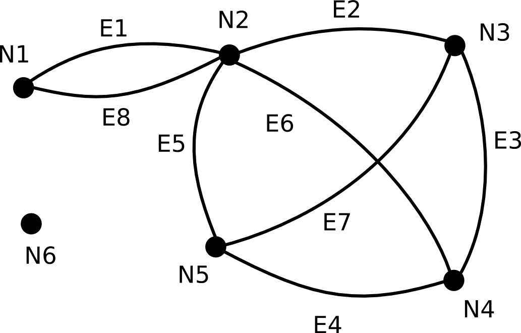
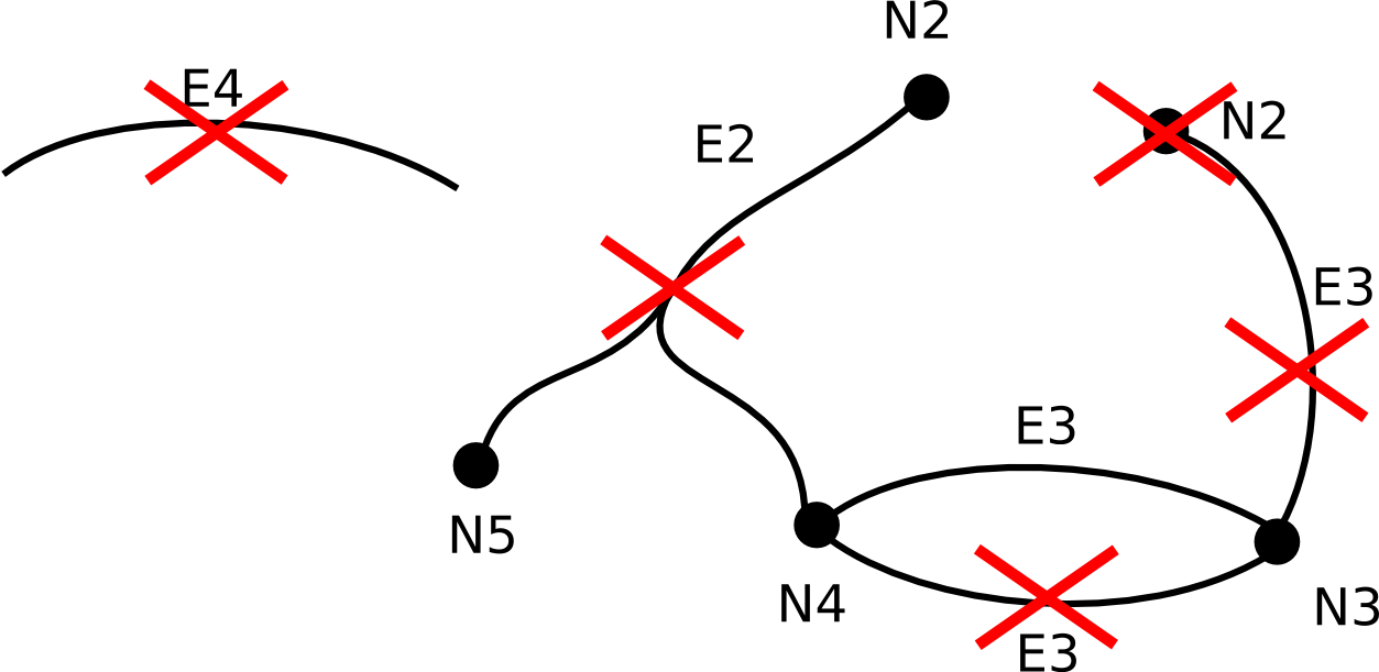
Figure Figure 1, “Example of a valid graph” shows a valid graph, figure Figure 2, “Invalid graph topologies” shows a summary of disallowed topologies.
Interfaces and implementations
There are two basic interfaces for manipulating graphs in LuciadLightspeed:
-
ILcdGraph, which provides methods for retrieving the elements of a graph (which nodes and edges it contains) and their topology (how they are connected to each other). -
ILcdEditableGraph, which extends ILcdGraph and provides extra functionality for adding and removing nodes and edges.
TLcdGraph implements both interfaces and acts as the default graph
class which can be used to represent graphs in network applications.
Working with edges and nodes
Every Java object can be an edge or a node: the Network API does not require any interface to be implemented or
super class to be extended, for an object to become a node or an edge. This makes the integration of the network
functionality in other components very easy. The meaning of an object (whether it is an edge or a node) is derived
from the context in which it is used: the signature of a method determines the actual interpretation of its arguments.
Every argument of a method in the Network API that is interpreted as a node or an edge, has a name containing 'edge'
or 'node', e.g. TLcdGraph.getOppositeNode(Object aEdge, Object aNode).
Be sure that the implementation of the equals (and thus hashCode) methods of your domain model
elements is valid: objects which are equal according to their equals method, will be treated as one
and the same node or edge object in the graph.
Routes
A common problem in network applications is to find the shortest route between two given nodes. Therefore,
the ILcdRoute interface and corresponding TLcdRoute implementation are provided to describe routes in a graph.
Definition and properties of routes
In mathematics, there are a lot of terms describing routes, depending on their properties. In LuciadLightspeed, we define a route in a very broad sense: every list of chained edges is considered as a route. The direction in which each edge is traversed, is determined by the order of the edges in the list.
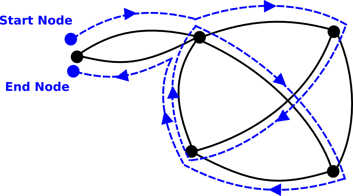
Figure Figure 3, “Example of a route (dotted lines) in a graph.” shows a route in one of its most general forms. Notice that:
-
an edge may be passed multiple times, even in the same direction
-
a node may be traversed multiple times
-
the edges of a route may cross each other
-
the route as a whole may be closed (i.e., its start and end node may be identical)
Interfaces and implementations
network provides one interface for representing routes: the interface ILcdRoute. It provides basic methods
for retrieving its edges and nodes.
TLcdRoute is the default implementation of this interface, and provides some methods for adding edges to a route.
An extra utility class provides functionality for analysis of routes, e.g., calculating the total value (distance, travelling time, …) of a route in a valued graph (see article Valued graphs).
Valued graphs
Most graphs have values associated with their edges, such as the distance of a road, the time to traverse a road or the length of a pipe. Sometimes values are also associated with nodes (e.g., the time to wait for a traffic light on a road junction). Even more complex associations are possible, such as values associated with a turn (a set of succeeding edges) in a graph. These values are often crucial in the algorithms we use in graph problems: finding the shortest route for example, requires knowing the distance of each edge in the graph. This article presents a set of interfaces and classes to incorporate those values in our graph model, in a way that makes them usable for the algorithms described in the next articles.
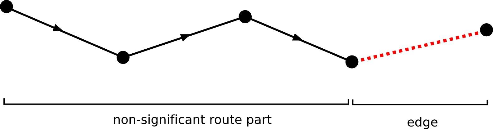
The route-based edge value function
As mentioned above, solving a tracing or routing problem, requires knowledge of the values associated with each edge, node and turn in the graph. As we will demonstrate further, all these types of association can be reduced to one general case: what is the value of an edge, given the route that was followed to reach that edge.
The networking and route planning component introduces an interface for a function that associates a value with an edge, given
the route followed to
reach that edge: ILcdEdgevaluefunction. This interface consists of two methods:
-
public double computeEdgeValue(ILcdGraph aGraph, ILcdRoute aPrecedingRoute, Object aEdge, TLcdTraversalDirection aTraversalDirection).The method takes the routeaPrecedingroutethat was followed to reach the edge (aEdge) and the edgeaEdgeas an argument, and returns the actual value associated withaEdge.In some algorithms, routes are calculated the inversed way, e.g. starting with the last edge of the route and working backwards until the start node is reached. This is where the
aTraversalDirectionargument comes in: it indicates the direction in which the edge is traversed. If equal toTLcdTraversalDirection.BACKWARD, the edge and the given preceding route will be traversed in opposite direction (the 'preceding' route becomes thus a succeeding route of the edge). Edge value functions should adapt their values accordingly. A comprehensive example is given in figure Figure 4, “Effect of the aTraversalDirection flag. The arrows indicate the direction that is used to determine the edge’s value.”.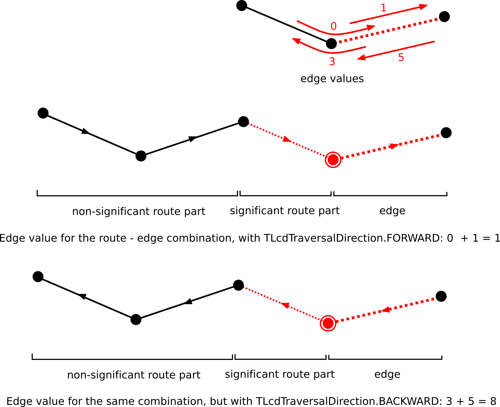 Figure 4. Effect of the aTraversalDirection flag. The arrows indicate the direction that is used to determine the edge’s value.
 -
public int getOrder():This method returns the order of this function. The order of an edge function is the maximum number of preceding edges that are taken into account when calculating an edge value. I.e., it indicates the maximum number of edges of the preceeding route that can have an impact on the actual result value associated with an edge. Note that overestimating the order will not influence the results of the algorithms provided in the networking and route planning component (although they can cause a severe performance penalty), but underestimation will.
Depending on your application, you will need a different implementation of this interface. In the next sections, we give an overview of the default implementations that are provided with LuciadLightspeed.
Simple edge value functions
A simple edge value function is an edge value function whose value, returned for a given edge, depends only on the edge itself and the direction in which it is traversed. Common examples are the length or the travel time of a road. The only element of the preceding route that has an influence on the value, is the end node of the route, as it determines the edge’s traversal direction. Since no edges are taken into account, the order of this function is 0.
The class ALcdSimpleEdgeValueFunction is an abstract class that implements the interface ILcdEdgevaluefunction. It has one abstract
method whose implementation returns the value associated with the given edge:
public abstract double computeEdgeValue(ILcdGraph aGraph, Object aEdge, TLcdTraversalDirection aTraversalDirection).
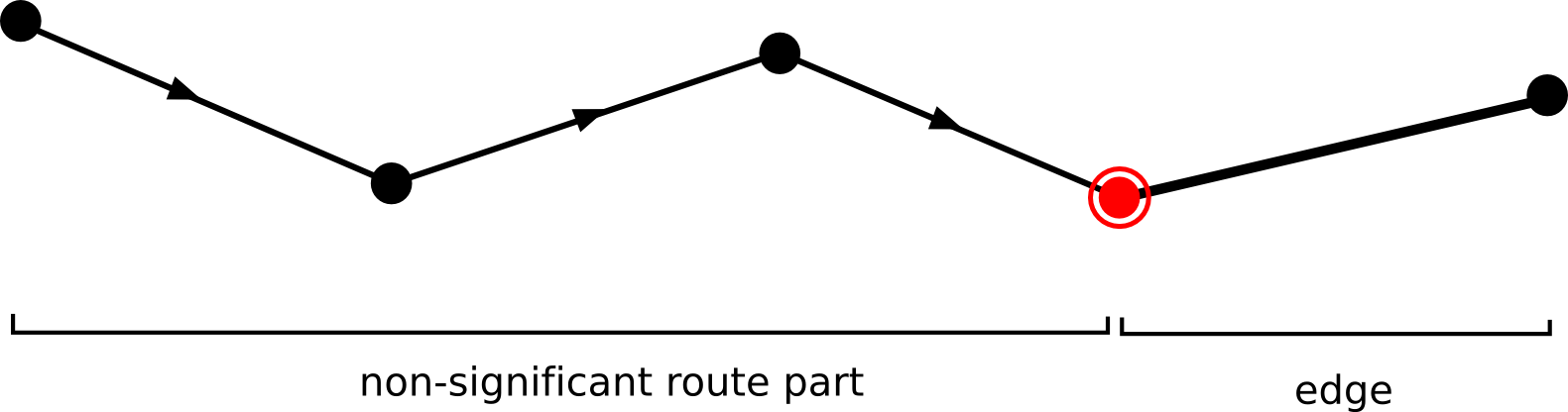
Node value functions
A node value function is an edge value function whose value, returned for a given edge, depends only on one node of that edge. The mean time to wait on a junction for a traffic light is a typical example. Since the node value is not influenced by any of the edges in the preceding route, the order of this function is 0.
ALcdNodeValueFunction is an abstract class that implements the interface ILcdEdgevaluefunction and provides one abstract method
whose implementation should return the value associated with the given node:
public abstract double getNodeValue(ILcdGraph aGraph, Object aNode)
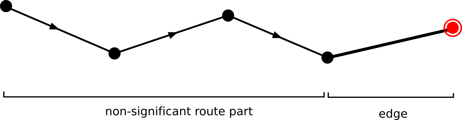
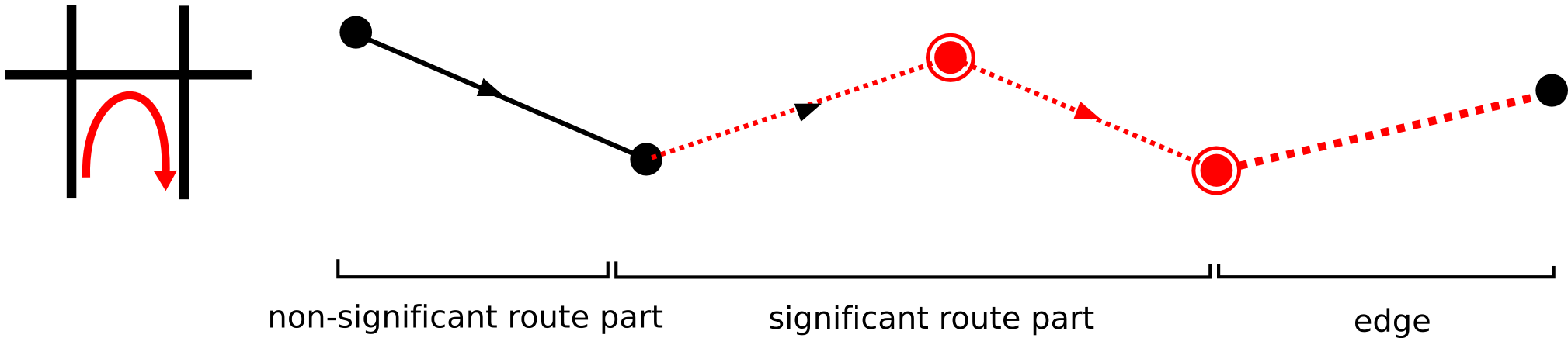
Note that this function returns a value for that node of the edge the is passed first (see figure Figure 6, “A node value function. The double-circled node indicates the information that is used to determine the edge value”). Although most of the time this
function will suffice, there could be situations where you will need the value for the second node (see figure Figure 7, “Another possible node value function.”).
Turn value functions
A turn value function is an edge value function whose value, returned for a given edge, depends only of that edge, the edge preceding it and the node connecting them. Since this function uses the last edge of the preceding route as a parameter, the order of this function is 1.
ALcdTurnValueFunction is an abstract class that implements the ILcdEdgevaluefunction interface and has one abstract method
whose implementation returns the value associated with the given turn:
public abstract double getTurnValue(ILcdGraph aGraph,
                                    Object aEdge,
                                    Object aNode,
                                    Object aNextEdge,
                                    TLcdTraversalDirection aTraversalDirection)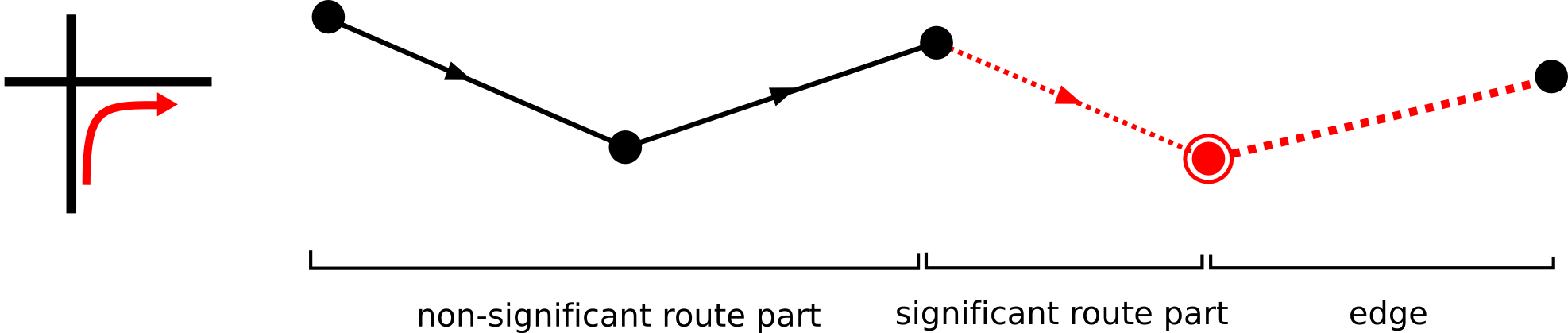
More complex functions
Sometimes you will need more complex functions. E.g., when modelling the cost of a U-turn in a roadmap, you will need the
last two edges of
the preceding route, and your function will have order 2 (see figure Figure 9, “A order-2 function that can be used to model U-turn costs.”). In these cases, you will need
to write your own implementation of ILcdEdgevaluefunction. Be sure to always return a correct value for the function order.
Composite functions
In some applications, an edge will have a cost that is a combination of two or more of the functions described above. A typical example is a roadmap, which combines road lengths with turn costs, and perhaps also the time to wait for a traffic light.
For these purposes, you can use the class TLcdCompositeEdgeValueFunction, which takes an array of edge functions
as its argument. The edge value that is returned by this function, is the sum of the edge values of all these edge function.
Functions
of different orders can be combined. The order of the composite function is the maximum order of all edge functions in the
array.
Modelling directed edges and turn restrictions
Until now, we never mentioned anything about directed edges (i.e. edges which can only be passed in one direction). Doing
this is very
easy: as described above, you can associate distinct values with an edge, depending on the direction in which it is traversed.
By assigning
the value Double.POSITIVE_INFINITY value to one of the directions of an edge, you make it untraversable in that direction, and the edge
becomes thus directed.
Turn restrictions can be modelled the same way: by associating a Double.POSITIVE_INFINITY value with a turn, the turn becomes
untraversable.
The distance function
Distance functions are functions that can calculate a distance between two nodes, or more general, between two given routes. Best known is the euclidean distance function, but other implementations are possible: the Manhattan distance function, time-based functions, roadmap-based distance functions, …
Distance functions are used in routing algorithms as a heuristic function, to speed up the routing process. Depending on the type of algorithm you use, extra constraints are put on the distance function (please refer to the API reference documentation for detailed information).
Similar to the edge value functions, the networking and route planning component provides an interface for distance functions,
ILcdDistanceFunction, with the
following two methods:
-
public double computeDistance(ILcdGraph aGraph, ILcdRoute aPrecedingRoute, ILcdRoute aSucceedingRoute, TLcdTraversalDirection
                                       aTraversalDirection)
. The value that is returned, is the distance between the end node ofaPrecedingRouteand the start node ofaSucceedinggRoute. -
public int getOrder(). The order has the same meaning as the edge value function’s order.
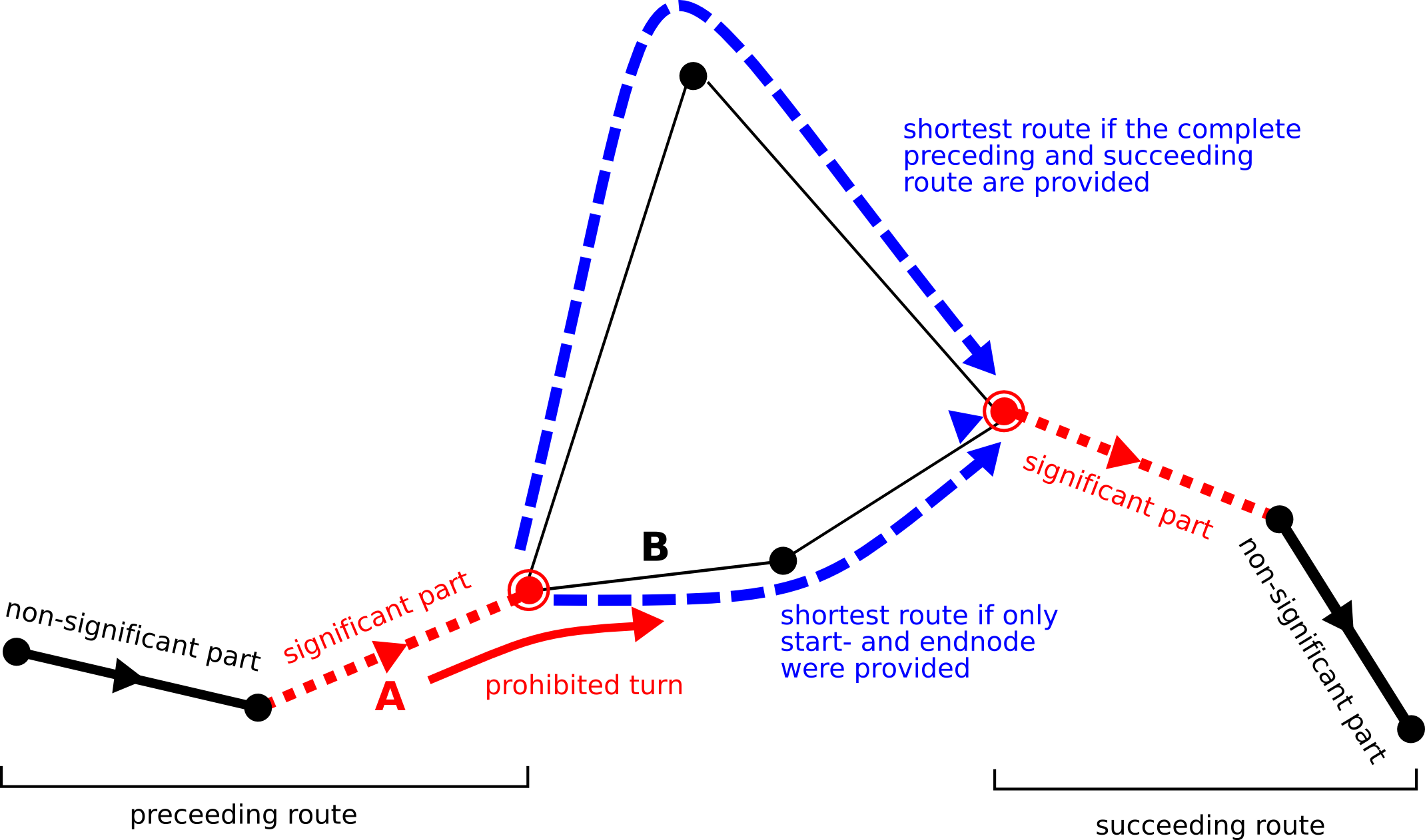
When using a simple euclidean distance function, only start and end node matter, but higher order functions require also preceding and succeeding edges to calculate the correct distance, therefore routes are used as arguments in this function. As an example, take a function that returns the distance of the shortest route between the two given routes as distance (see figure Figure 10, “Example of a routing problem. A turn restriction between edge A and B is added, which means it is prohibited to traverse edge B when coming from edge A.”).
One extra class is provided, ALcdNodeDistanceFunction, which can be used to implement simple functions of order 0, which compute
distances between two nodes.
Solving shortest route problems
Besides basic graph representation classes and interfaces, LuciadLightspeed provides several algorithms, from which the shortest route algorithm is the most important.
Definition of the shortest route problem
The shortest route problem tries to find for two given nodes, or more general, two given routes, the shortest route between them. The value of the shortest route equals the sum of values corresponding to each edge in the path. These edge values will be provided by a edge edge value function, as described in article Valued graphs.
Figure Figure 10, “Example of a routing problem. A turn restriction between edge A and B is added, which means it is prohibited to traverse edge B when coming from edge A.” shows a small example: the edge length is used as the edge value function, but a turn restriction (see figure) is added to the graph. The edge value function thus has order 1. The example shows that providing only a start node and end node is not enough to get a correct result, when using an edge value function with order > 0.
Interfaces and implementations
ILcdShortestRouteAlgorithm defines an interface for shortest route algorithms. It offers one method with the following signature:
public ILcdRoute getShortestRoute(ILcdGraph aGraph,
                                  ILcdRoute aPreceedingRoute,
                                  ILcdRoute aSucceedingRoute,
                                  ILcdEdgeValueFunction aEdgeValueFunction,
                                  ILcdDistanceFunction aHeuristicDistanceFunction).
The method getShortestRoute takes a preceding and
succeeding route, an edge value function and a heuristic distance function as a argument.
It is not required to provide a heuristic function, but the effect on performance of a good heuristic function is significant. Be sure that your heuristic function will never overestimate the effective distance between two routes, otherwise the validity of the results of the algorithms cannot be guaranteed. An euclidean distance function is an example of a good heuristic function: it is a good indicator of the remaining distance, while it never exceeds that distance (there exists no shorter route than a straight-line between start- and endpoint).
TLcdRouting is the default implementation provided with LuciadLightspeed. The algorithm used was inspired by the well-known Dijkstra
and A* algorithms,
which were significantly adapted to handle advanced edge value functions and heuristic distance functions. It should fit the
need of most routing applications.
Solving tracing problems
Definition of the tracing problem
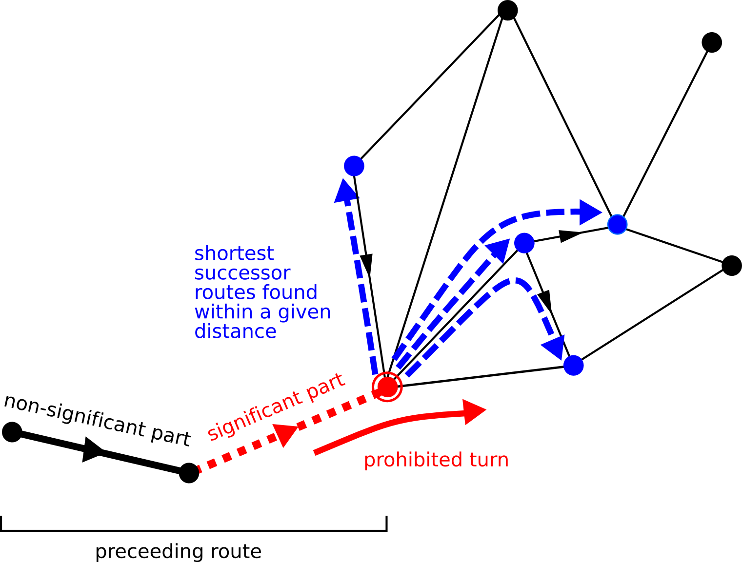
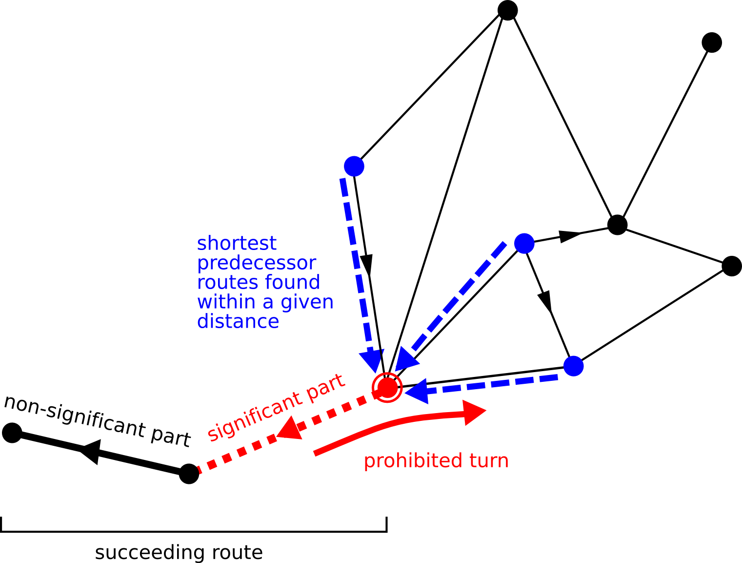
While the routing algorithm finds the shortest route between two routes, the tracing algorithm finds all nodes within a certain distance of a node, and their shortest routes from/to that node. Searching for a contamination source in a pipeline or a river is a typical example of a tracing application. In order to take care of turn restrictions, the same generalization is made as in the routing problem: instead of a node, a whole route is provided as an argument.
There are two variants of the tracing problem: searching for all predecessors, and searching for all successors. The difference between the two is shown in the example below.
Interfaces and implementations
LuciadLightspeed provides the interface ILcdTracingAlgorithm for tracing algorithms. The interface offers the following two methods:
public void getPredecessors(ILcdGraph aGraph,
                            ILcdRoute aSucceedingRoute,
                            ILcdEdgeValueFunction aEdgeValueFunction,
                            ILcdTracingResultHandler aResultHandler,
                            double aDistance)
public void getSuccessors(ILcdGraph aGraph,
ILcdRoute aPreceedingRoute,
ILcdEdgeValueFunction aEdgeValueFunction,
ILcdTracingResultHandler aResultHandler,
double aDistance)The TLcdTracing class is is the default implementation for tracing.
The interface ILcdTracingResultHandler should be implemented by the user of the algorithm. Its interface offers only one method:
public void handleNode(Object aNode,
                       ILcdRoute aShortestRoute,
                       double aDistance);
This method is invoked by the tracing algorithm for every node that is found within the tracing distance. It provides the node that is found, the shortest route to reach that node, and its distance. The user should do what is appropriate in this method to handle the result, e.g., storing the routes or highlighting them on a map.
Partitioned graphs
Planning routes in real-world networks, consisting of millions of edges and nodes, can take very long with the default routing algorithm, and requires large amounts of memory. Partitioning and prerouting graphs can reduce the routing time in large graphs significantly, as well as the memory usage. This article explains the basic partitioning API, while the next two articles focus on partitioning algorithms and prerouting.
Definitions and properties of partitioned graphs
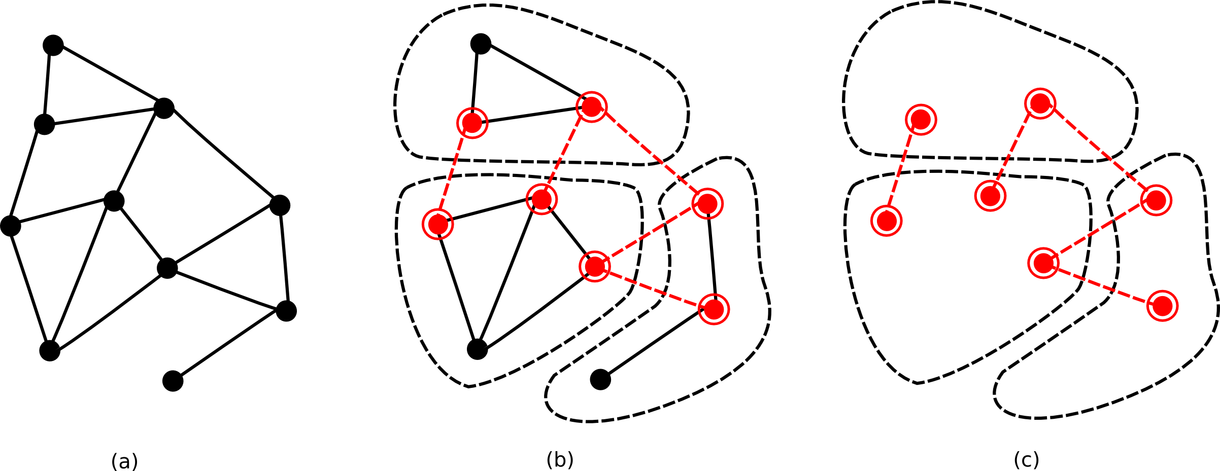
A partitioned graph is a graph in which the nodes of the graph are grouped together in two or more partitions. Each partition on itself is a graph, and all partitions together form the partitioned graph. Figure Figure 13, “(a) the original graph, (b) a partitioned version of the graph, and (c) its corresponding boundary graph. The dotted lines are boundary edges, the double-circled nodes are boundary nodes.” shows an example of a partitioned graph.
The partitioned structure introduces two kind of edges: internal edges and boundary edges. The internal edges of a partition are all edges that connect nodes in the same partition, while the boundary edges are all edges that connect nodes in different partition. Nodes connected to at least one boundary edge are called boundary nodes, all other nodes are internal nodes. The boundary edges of all partitions in a partitioned graph, together with their boundary nodes, form the boundary graph of that partitioned graph.
Since each partition is a graph, and the partitioned graph on itself is also a graph, all invariants that hold for a normal graph (see Definition and properties of graphs), should also hold for each partition, as well as for the partitioned graph. E.g., this implies that a node can be part of at most one partition, as it can be contained in the partitioned graph only once.
Interfaces and implementations
The partitioning package extends the graph package with a number of classes and interfaces, providing support for partitioned graphs:
-
ILcdPartitionedGraphextendsILcdGraphand offers extra functionality for inspecting the partitions and boundary graph of partitioned graphs. -
ILcdLimitedEditablePartitionedGraphis anILcdPartitionedGraphwith the possibility to add and remove partitions and/or boundary edges, but not to add or remove edges or nodes from/to the child partitions (it does not prohibit however the posibility to add or remove edges and nodes to child partitions directly). -
TLcdLimitedEditablePartitionedGraphis the default implementation ofILcdLimitedEditablePartitionedGraph. -
TLcdPartitionedGraphis an extension ofTLcdLimitedEditablePartitionedGraphthat additionally implementsILcdEditableGraph. It is a partitioned graph that is fully editable, i.e. a graph to which partitions can be added (and removed), as well as edges and nodes. ItsaddNode(Node aNode)method implements a node assignment policy to decide in which partition a new node should be added. It can be overwritten in subclasses to use a more adequate assignment policy.
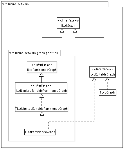
Figure Figure 14, “The structure of the basic network.graph packages.” gives an overview of the class hierarchy of the network.graph and network.graph.partition packages.
Partitioned Routing
Overview
In article Partitioned graphs, it was already mentioned that partitioning graphs can increase performance and reduce memory when routing. LuciadLightspeed offers an advanced routing algorithm that takes advantage of partitioned graphs and provides faster and less resource-demanding routing in large graphs.
This partitioned routing algorithm makes use of precomputed distance tables, to accelerate the routing process. A distance table is a simple table, containing the distances of all shortest routes between every two boundary nodes in a partition. There is one distance table for each partition. Distance tables can be precomputed by a special preprocessor, that calculates all shortest routes between every two boundary nodes in each partition with the default routing algorithm.
Note that distance tables are specific to the edge value function that is used: the shortest route distances in the tables depend on the edge value function, and thus, changing the edge value function requires recomputing the distance tables.
Interfaces and implementations
-
TLcdPartitionedShortestRouteAlgorithmis an implementation ofILcdShortestRouteAlgorithm, based on the partitioning an preprocessing of graphs to increase performance and reduce memory usage. It requires anILcdShortestRouteDistanceTableProvider, which provides the distance tables for all partitions in the partitioned graph. -
ILcdShortestRouteDistanceTableProviderdefines an interface for accessing distance tables. It provides methods for mapping partitions on distance tables and vice versa. -
TLcdShortestRouteDistanceTableProvideris the default implementation ofILcdShortestRouteDistanceTableProvider. -
TLcdPartitionedShortestRoutePreprocessoris the preprocessor for the partitioned routing algorithm. It takes anILcdShortestRouteDistanceTableProvideras an argument to store the resulting distance tables. -
ILcdShortestRouteDistanceTablerepresents a distance table, containing the set of boundary nodes for one partition and all shortest route distances between them. -
TLcdShortestRouteDistanceTableis the default implementation ofILcdShortestRouteDistanceTable.
Partitioning algorithms
Partitioning strategies
Graphs can be partitioned in many different ways. Partitioning criteria can be based, for example, on the geographical position of the nodes, on the road type of the edges, or other criteria. In general, the partitioning strategy will be dependent of the target application.
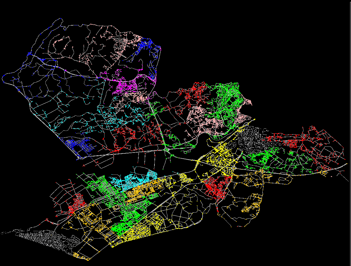
In theory, every partitioning scheme can be used for the partitioned routing algorithm described in the previous article. But in order to result in a performance increase and/or memory reduction, a specific criterium should be used, based on the coherence and connectivity of the edges and nodes: tightly connected areas, like a city center, should preferably be grouped together in one partition, while loosely coupled areas, like two city parts separated by a river, should preferably be divided in two separate partitions. Figure Figure 15, “An example of a partitioned graph.” gives a sample partitioning scheme of a city, based on such a criterium.
Interfaces and implementations
The network.algorithm.partitioning package offers support for partitioning graphs.
The interface ILcdPartitioningAlgorithm acts as a general interface for partitioning algoirthms, taking an ILcdGraph as input and ILcdPartitionedGraph as output.
Currently, one implementation is provided, TLcdClusteredPartitioningAlgorithm, which uses a criterium based on graph coherence, as described above. In addition to the default partitioning, one can pass
a list of constrainted edges to the algorithm, which contains all edges that may not become boundary edges within the generated
partitioned graph.
A parameter can be set to specify the number of iterations to be done by the algorithm - the more iterations, the better the
partitioning result will be. For small graphs, the algorithm can become unstable, resulting in a partitioning scheme where
each node is a separate partition.
Manual partitioning
It is not always possible to load a whole graph into memory, in which case the TLcdClusteredPartitioningAlgorithm
cannot be used. In these cases, a first manual partitioning step should be performed to split up the
top-level graph in a few smaller, manageable partitions, before the TLcdClusteredPartitioningAlgorithm
can take over to create additional partitioning levels.
A good manual partitioning criterium should meet two requirements:
-
It can be used locally (no need to load the full graph to know in which partition a node will reside)
-
It takes into account the algorithms that will use it. In case of partitioned routing, this means that the resulting partitions should be highly clustered (minimal number of boundary nodes and edges).
A simple criterium would be to create partitions based on rectangular bounds. This criterium can be used locally (for each node or edge, a simple contains test determines in which partition it is located), but doesn’t always deliver good results for the second requirement: whenever the bounds cross a highly clustered area, this will result in a lot of boundary nodes and edges.
A more advanced criterium is the natural structure that is present in the data. This could be the file structure, an administrative structure (county, state, country, …) or any other structure associated with the data. These criteriums often result in fairly good partitioning schema’s, since these structures are also often driven by a sort of clustering requirement.
For example, a road network can be partitioned based on the country to which they belong; it almost never happens that a country border crosses a city center, and most countries have only a limited number of connections with neighbouring countries. This makes the country structure an excellent criterium for a first, high-level partitioning schema.
Numeric Graphs
Graphs are often too large to be completely contained in memory. Writing a custom partitioned graph decoder and encoder with on-the-fly loading and performant graph queries can be difficult and time-consuming. Numeric graphs provide an alternative solution, relieving the developer of the burden of implementing his own graph.
Numeric graphs have several advantages over other graphs:
-
They are very compact in memory: all graph objects (edges, nodes, partitions) are represented by a single long value.
-
They can be stored on disk even more compact.
-
They are very fast to query (partition containment, connectivity, edge values).
-
They are very well suited for on-the-fly loading.
Due to their superior performance, numeric graphs should be considered whenever graphs become too large to be contained completely in memory, or performance of algorithms applied on them is not sufficient.
Interfaces and implementations
The following classes and interfaces are provided in the network.numeric package:
-
TLcdNumericGraphrepresents a numeric graph. All algorithmic computations will be done on this graph. This graph also provides access to its edge value function and distance table provider. -
TLcdNumericGraphEncoderis an encoder for converting graphs to a numeric graph, and writing them to disk. It can encode the topology of a graph, its edge value function and will also preprocess the graph and encode the resulting distance tables. -
TLcdNumericGraphDecoderis a decoder for reading numeric graph files, supporting on-the-fly loading. -
ILcdNumericGraphMappingHandleris a callback interface that will be called byTLcdNumericGraphEncoderfor every partition, node and edge that is mapped on a numerical identifier.
Numeric graph file structure
As explained in section Interfaces and implementations, the numeric graph encoder encodes not only a graph’s topology, but also the edge value function and distance tables.
This results in 3 different file types:
-
Topology files (*.ng): these are the main graph files, containing the partitioned structure and topology of the graph. A graph might be split up into multiple topology files, to keep the file size manageable.
-
Edge value files (*.ngv): next to each topology file, an edge value file is stored per edge value function, containing the positive and negative edge values for all edges, for that function. Multiple edge value functions may be encoded for the same numeric graph.
-
Distance tables (*.ngd): next to each edge value file, a distance table file is stored, containing the corresponding distance tables.
Adjusting the file size and number of files
Although numeric graphs are much more compact than normal graphs, even very large numeric graphs can be too large to fit in memory. Splitting up numeric graph files in multiple smaller files allows on-the-fly loading of partitions, which is faster and consumes less memory, as unused parts of the graph won’t be loaded. Splitting is done based on the partitioning schema.
The number and size of the graph files can be tweaked via the node split threshold parameter on the
TLcdNumericGraphEncoder. This parameter allows to specify for each hierarchical level in the graph
the number of nodes a partition should minimally have to be written to a separate file.
Working with numeric graphs
Converting a dataset into a numeric graaph
The following steps summarize the complete workflow from original data to numeric graph:
-
Load the original data describing the network into an
ILcdModel, using anILcdModelDecoder. -
Convert the data to an
ILcdGraph. -
Partition the graph (may be in multiple levels) using the
TLcdClusteredPartitioningAlgorithmor custom partitioning algorithms. If the graph is to large to be handled by theTLcdClusteredPartitioningAlgorithm, it might be necessary to perform a first partitioning step manually (see section Manual partitioning for more information). -
Write an
ILcdEdgevaluefunction(based on the geometry and attributes of the edges in the graph). -
Convert the partitioned graph together with the edge value function into a numeric graph and write it to disk, using
TLcdNumericGraphEncoder. The encoder will automatically compute and encode the shortest route distance tables as well.
Steps 1-4 were already explained in detail in the previous sections.
The last step, the conversion of the graph to a numeric graph, is illustrated in the code snippet below. The numeric graph encoder performs the mapping from graph to numeric graph , preprocesses the graph and encodes the graph’s topology, edge values and distance tables. The snippet continues on the sample introduced in the Working with large graphs tutorial.
String tmpDir = System.getProperty("java.io.tmpdir");
String graphDest = tmpDir + File.separator + "graph.ng";
String valuesDest = tmpDir + File.separator + "graph.ngv";

TLcdNumericGraphEncoder encoder = new TLcdNumericGraphEncoder();
encoder.exportGraph(partitionedGraph,
                    edgeValueFunction,
                    mappingHandler,
                    graphDest,
                    valuesDest);
The mapping handler will be called to report every mapping from a native node or edge in the original graph to a corresponding numerical identifier in the numeric graph. These mappings will be needed in the next step, to switch between native and numeric graph representation.
The mapping information can either be stored on the domain objects, or, if this is not possible, in a separate look-up table, as illustrated in the code snippet below.
Map<TLcdXYPoint, Long> node2idMap = new HashMap<>();
Map<Long, TLcdXYLine> id2edgeMap = new HashMap<>();

ILcdNumericGraphMappingHandler<TLcdXYPoint, TLcdXYLine> mappingHandler = new ILcdNumericGraphMappingHandler<TLcdXYPoint, TLcdXYLine>() {
  @Override
  public void mapGraph(ILcdGraph<TLcdXYPoint, TLcdXYLine> aGraph, long aNumericId) {
  }

  @Override
  public void mapNode(TLcdXYPoint aNode, long aNumericId) {
    node2idMap.put(aNode, aNumericId);
  }

  @Override
  public void mapEdge(TLcdXYLine aEdge, long aNumericId) {
    id2edgeMap.put(aNumericId, aEdge);
  }

  @Override
  public void mapBoundaryEdge(TLcdXYLine aBoundaryEdge, long aNumericId) {
    id2edgeMap.put(aNumericId, aBoundaryEdge);
  }
};
Computing shortest routes on graphs
After the graph has been exported to a numeric graph, it can be decoded again with the numeric graph decoder. Large partitions in separate files will be automatically loaded on-the-fly.
TLcdNumericGraphDecoder decoder = new TLcdNumericGraphDecoder();
TLcdNumericGraph numericGraph = decoder.decodeGraph(graphDest, valuesDest);
To perform a query on the graph, the native nodes and edges involved in the query must first be mapped on their numeric counterpart. This can be done using the mapping that was built during the encoding. The mapped nodes can be used to create a numeric route.
TLcdRoute<Long, Long> precedingNumericRoute = new TLcdRoute<>(numericGraph, node2idMap.get(startNode));
TLcdRoute<Long, Long> succeedingNumericRoute = new TLcdRoute<>(numericGraph, node2idMap.get(endNode));
Once the mapping to numeric edges and nodes has been done, the routing can be done the same way as with a normal graph. The edge value function and distance tables are retrieved from the numeric graph.
TLcdPartitionedShortestRouteAlgorithm numericRouteAlgorithm = new TLcdPartitionedShortestRouteAlgorithm();
numericRouteAlgorithm.setDistanceTableProvider(numericGraph.getShortestRouteDistanceTableProvider());
ILcdRoute<Long, Long> numericRoute = numericRouteAlgorithm.getShortestRoute(numericGraph,
                                                                            precedingNumericRoute,
                                                                            succeedingNumericRoute,
                                                                            numericGraph.getEdgeValueFunction(),
                                                                            null);
After the shortest route has been found, the numeric edges in the route should be mapped back to native edges. This can be done again using the mapping that was created during the encoding, but now in the other direction.
for (int i = 0; i < numericRoute.getEdgeCount(); i++) {
  System.out.println("Shortest route edge " + i + ": " + id2edgeMap.get(numericRoute.getEdge(i)));
}
Working with multiple edge value functions
Multiple edge value functions may be associated with a numeric graph. Once a graph has been exported
to a numeric graph, the TLcdNumericGraphEncoder.exportEdgeValueFunction method may be called
to export additional edge value functions. This method will only encode the additional edge value
function, and leave the original topology files untouched.
The TLcdNumericGraphDecoder has a decodeGraph method wit a aGraphEdgeValuesSource parameter
which allows to specify which edge value function should be loaded with the numeric graph. The decoder
can decode only one edge value function per numeric graph instance.
Adjusting numeric graphs
After a graph has been converted to a numeric graph, a few edit operations can still be performed on the numeric graph:
-
adding nodes
-
adding edges
-
changing edge value functions
The TLcdNumericGraphEncoder.saveGraph method should be called to write graph changes to disk.
This method is optimized to write only those files containing partitions that have changed.
Whenever an edge is added to a numeric graph or an edge value has been updated, the distance tables of all partitions that
are involved in the change will be discarded (the distance table provider will return null for these
partitions). These distance tables will be lazily recomputed when requested.
Adding nodes and edges
Adding nodes and edges can be done via the addNode and addEdge operations on TLcdNumericGraph.
When a new node or edge is added, these methods will return the new numerical id corresponding with
the new node or edge.
The add operations are intended to be used only sporadically: there is only space for a limited number
of extra edges and nodes once a graph has been converted to a numeric graph. This number can be
configured via the setExpansionSize method of the TLcdNumericGraphEncoder. The structure of
the numeric graph will also be less optimal for edges which are added after the graph has been
converted (however, if the number of added edges is only small, this won’t affect performance).
When a large number of edges and/or nodes needs to be added, it is advised to update the original graph
and convert it to a numeric graph again.
The edge values for all newly added edges are initialized to Double.POSITIVE_INFINITY.
Removing edges
Removing edges is not possible, but can be emulated by setting the edge value to
Double.POSITIVE_INFINITY.
Updating edge value functions
Changing edge values can be done via the updateEdgeValue method on TLcdNumericGraph.
There are no restrictions on changing the edge value functions.
Cross Country Movement
Cross country movement is the planning of routes across an area, without restriction to a particular set of nodes and edges. Although this problem could be solved using the standard shortest route algorithm by discretizing the area, this would require a large amount of memory to get a sufficiently accurate solution. The cross country algorithms are specifically designed to solve this problem and hence require significantly less memory and time. The rest of this article explains the basic cross country movement API and how to use it effectively.
Interfaces and implementations
-
TLcdCrossCountryShortestRouteAlgorithmis the default algorithm to solve a cross country movement problem. -
ILcdCrossCountryDistanceFunctiondefines an interface for computing distances in an area. -
ALcdCrossCountryRasterDistanceFunctionis an implementation ofILcdCrossCountryDistanceFunctionfor computing distances on anILcdRaster.
Using the algorithm
The construction of a TLcdCrossCountryShortestRouteAlgorithm requires specifying a horizontal and vertical discretization step. A smaller step will result in a more accurate solution
but also increases the computation time. A common case is that the route is computed on an ILcdRaster. If this is the case a discretization step size equal to (a multiple of) the distance between 2 neighboring raster values
is a good choice.
To compute a route you must specify the start point, end point and distance function. In addition you can also optionally specify a heuristic distance function. Using a heuristic distance function can significantly speed up the algorithm so you should specify one if possible. However, to guarantee a valid result this function must always underestimate the real distance as computed by the specified distance function.