What happens?
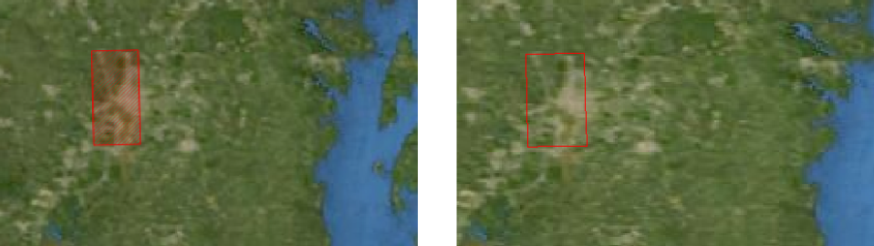
Your imagery layer displays a red hatched rectangle instead of any actual imagery data. You see this rectangular box when you have zoomed out to a fair distance from the data.
Why does this happen?
The red rectangle is a placeholder for the actual data, and indicates the position of the data on the map. The placeholder protects you from loading too much imagery data.
Suppose that you have a 100 MB imagery file that covers a small city, a GeoTIFF file for instance. You load the file on your map while you’re zoomed out far enough to see an entire continent. At that point, the area covered by the image corresponds to only a small part of your screen, say 20x20 px (pixels). To render those 20x20 pixels, the rendering engine would have to load the whole file - 100 MB. That would be fine if it were the only thing it had to do, but you probably have lots of other data sets to handle as well. From that zooming distance, you wouldn’t be able to see any meaningful detail of the imagery anyway.
That’s why the default LuciadCPillar settings prevent the data from loading. LuciadCPillar shows a placeholder rectangle instead of the actual data.
How can you prevent this?
To make the rectangle go away and see your imagery, you have a couple of options:
Simply zoom in
Zoom in to make your imagery data visible. Suppose you zoom to the street level of the city imagery file. Your entire view now holds relevant data, 1000 x 1000 px for instance. You see just a small portion of the data, though, namely the part that surrounds the street you’re looking at. Remember, the file covers an entire city. Let’s say the rendering engine now only has to load 3000 x 3000 px from the data. That means the start resolution factor (3000x3000) / (1000x1000) becomes 9, a much more realistic value. Loading the data makes sense now.
Use multi-leveled imagery data
Instead of using a single, huge 30.000 x 30.000 px image, you store extra lower-resolution images in the same file. This is called multi-leveling. You add a 10.000 x 10.000 px image and a 3000 x 3000 px image, for example. The rendering engine automatically picks the most appropriate level for the zoom level of the map user, so multi-leveling an image can drastically increase efficiency. If the rendering engine can use the 3000 x 3000 image instead of the 30.000 x 30.000 image, it becomes 100 times more efficient. The more levels you add, the more efficient it can be. Data sets covering the entire world, such as Bing maps imagery, have over 20 levels. Common imagery formats such as GeoTIFF support multi-leveling, while others such as PNG or JPG don’t. See Using GDAL to convert your image to a multi-level image for more detailed instructions.
Using GDAL to convert your image to a multi-level image
GDAL is an open-source GIS library that you can use to convert an image to a multi-leveled, tiled and compressed image. Such images offer the best possible performance when they’re visualized in a LuciadCPillar application, or when they’re served over WMTS through LuciadFusion. You can optimize color images and measurement images with GDAL.
Optimizing a color image
If your image contains colors, you can use the following GDAL code:
gdal_translate -co compress=jpeg -co tiled=yes -co blockxsize=256 -co blockysize=256 ${INPUT_FILE} ${OUTPUT_FILE}
gdaladdo -r average ${OUTPUT_FILE} 2 4 8 16
-
gdal_translate tiles and compresses the data. In this example, we use JPEG compression and tile the data in 256 x 256 tiles.
-
gdaladdo adds overview levels to an existing file.
-
The extra levels take the average of pixels, for smooth results.
-
We generate 4 extra levels in the example, to have 5 in total. The resolutions are 1/2, 1/4, 1/8, 1/16 along each dimension. The number of pixels goes down by a factor of 4.
-
A good choice for the number of levels is:
log2(total_resolution/desired_resolution).
For example, for an image of 10kx10k:
log2(10k/1024) = 3.3 → 3 or 4 levels in total.
-
Optimizing a measurement image
If your image contains measurement values, such as elevation data, multi-band data, and hyperspectral data, you can use this GDAL code:
gdal_translate -co compress=LZW -co predictor=2 -co tiled= yes -co blockxsize=128 -co blockysize=128 ${INPUT_FILE} ${OUTPUT_FILE}
gdaladdo -r nearest ${OUTPUT_FILE} 2 4 8 16
-
gdal_translate tiles and compresses the data. In this example, we use LZW compression and tile the data in 128 x 128 tiles.
-
gdaladdo adds overview levels to an existing file.
-
The extra levels take the nearest of pixels. This approach results in more aliasing, but prevents interpolating values.
-
We generate 4 extra levels in the example, to have 5 in total. The resolutions are 1/2, 1/4, 1/8, 1/16 along each dimension. The number of pixels goes down by a factor of 4.
-
A good choice for the number of levels is:
log2(total_resolution/desired_resolution).
For example, for an image of 10kx10k:
log2(10k/1024) = 3.3 → 3 or 4 levels in total.
-